## Hidden Markov Models (HMMs)  Note: HMMs are well-known for their effectiveness in modeling the correlations between adjacent symbols, domains, or events, and they have been extensively used in various fields, especially in speech recognition and digital communication. Considering the remarkable success of HMMs in engineering, it is no surprise that a wide range of problems in biological sequence analysis have also benefited from them. --- ## What do you remember about dynamic programming? What is dynamic programming really? - introduced in 1950s by Richard Bellman of Rand Corp <!-- .element : class="fragment" data-fragment-index="1" --> <!-- .element : class="fragment" data-fragment-index="1" --> - it's hard to define <!-- .element : class="fragment" data-fragment-index="1" --> - it's extremely broad <!-- .element : class="fragment" data-fragment-index="1" --> [The theory of dynamic programming](https://www.ams.org/journals/bull/1954-60-06/S0002-9904-1954-09848-8/) <!-- .element : class="fragment" data-fragment-index="1" --> --- ## The setting 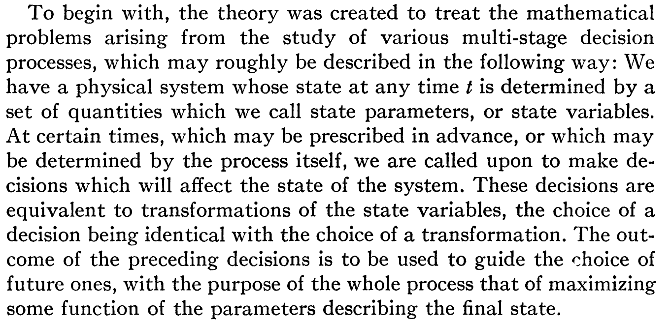 --- ## The insight 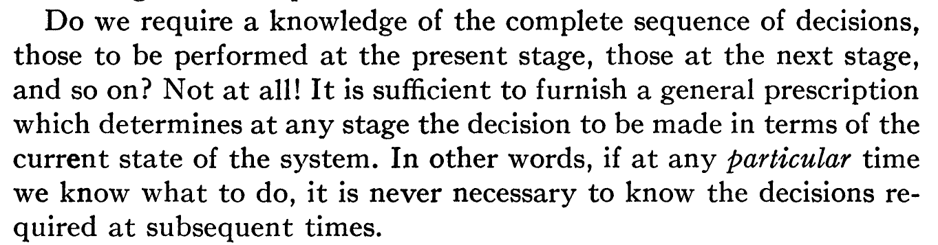 The essence of dynamic programming is "do the best you can from where you are" <!-- .element : class="fragment" --> --- Consider a process determined at any time by an M-dimensional vector $$ \mathbf{p} = (x_0, x_1, x_2, ..., x_m) $$ Consider a set of transformations $\mathbf{T} = { T_k }$, which are functions that transform $\mathbf{p}$ $$ T_k(p) = p' $$ We want to maximize our "return" -- the output of some scalar function $R(p)$ of the final state. --- We want to select a series of transformations, called "policy" $P=(T_1, T_2, ... T_N)$, which will yield successive states: $$ p_1 = T_1(p_0) \\\\ p_2 = T_2(p_1) \\\\ ...... \\\\ p_N = T_N(p_{N-1}) $$ The maximum value of $R(P_N)$, determined by an optimal policy, will only be a function of the initial vector $p_0$ and the number of stages N. The optimal return value is: $$ f_N(p) = Max_{P}R(p_N) $$ --- $$ f_N(p) = Max_{P}R(p_N) $$ Choose our first transformation $T_1(p_0)$. The maximum return from the following (N-1) stages is by definition: $$ f_{N-1}(T_1(p_0)) \\\\ = f_{N-1}(p_1) $$ Thus: $$ f_N(p) = Max_{P}R(p_N) = Max_{k} f_{N-1}(T_k(p)) $$ Which means: at any given time, we must choose the transformation that maximizes the return. --- ## Dynamic programming: the gist You have a sequence of states, and at each time step, you make a decision. You want to end optimally, for some definition of optimal. The brute-force way is to consider all possible sequences of decisions and then pick the best one, but this is not possible for long sequences with many possible decisions. <!-- .element : class="fragment" --> Instead, divide the problem into sub-problems: At any particular time determining your decision payoff depends only on the current state of the system, not on later states of the system. <!-- .element : class="fragment" --> This concept can apply to a huge array of problems, from investing to aircraft control to...computational biology. <!-- .element : class="fragment" --> --- ## A toy HMM for 5′ splice site recognition  <small>From: [What is a hidden Markov model?](https://www.nature.com/articles/nbt1004-1315) Don't confuse a state-space diagram with a [graphical model diagram](https://bmcmedresmethodol.biomedcentral.com/articles/10.1186/s12874-018-0629-0/figures/2) </small> Note: Often, biological sequence analysis is just a matter of putting the right label on each residue. In gene identification, we want to label nucleotides as exons, introns, or intergenic sequence. In sequence alignment, we want to associate residues in a query sequence with homologous residues in a target database sequence. We can always write an ad hoc program for any given problem, but the same frustrating issues will always recur. One is that we want to incorporate heterogeneous sources of information. A genefinder, for instance, ought to combine splice-site consensus, codon bias, exon/ intron length preferences and open reading frame analysis into one scoring system. How should these parameters be set? How should different kinds of information be weighted? A second issue is to interpret results probabilistically. Finding a best scoring answer is one thing, but what does the score mean, and how confident are we that the best scoring answer is correct? A third issue is extensibility. The moment we perfect our ad hoc genefinder, we wish we had also modeled translational initiation consensus, alternative splicing and a polyadenylation signal. Too often, piling more reality onto a fragile ad hoc program makes it collapse under its own weight. --- ## Hidden Markov Models (HMMs) * Provide a foundation for probabilistic models of linear sequence ‘labeling’ problems * Can be designed just by drawing a graph diagram * Originally developed for applications to voice recognition * Applications include: Gene prediction, protein secondary structure prediction, copy-number variation, chromatin-state assignment, chromatin topology ... Note: Joint probability $P(A,B) = P(A|B) P(B) = P(B|A) P(A)$, Marginal probability $P(X=A) = \sum_y P(X=A, Y=y_i)$ --- ## Markov models ## ↓ ## Hidden Markov models --- ## Markov Models * Set of states: $S \in {s_1, s_2, \ldots, s_n}$ * Process moves from one state to another generating a sequence of $L$ states: $x_{1}, x_{2}, \ldots, x_{L}, $ * Markov property: The probability of a symbol depends only on the preceding symbol, not the entire previous sequence $$P(x_{L} = s|x_{1},x_{2},\ldots,x_{i(L-1)}) = P(x_{L}=s|x_{i(L-1)})$$ * A Markov chain is defined by: * transition probabilities $a_{st} = P(x_i=t| x_{i-1}=s)$, $A=\\{a_{ij}\\}$ * initial probabilities: $a_{0s} = P(x_1=s)$ --- ## Example  <!-- .element width="80%" height="80%" --> $A = \begin{bmatrix} 0.7 & 0.3\\\\\\ 0.4 & 0.6 \end{bmatrix}$, $a_{0s} = (0.4, 0.6)$ Note: So let's consider I have two coins, one of them is fair and the other one is loaded. --- ## Calculation of sequence probability Multiplication Rule of probability: $$ P(A, B) = P(A|B) P(B) $$ $$ \begin{eqnarray} P(x_{1}, \ldots, x_{L}) &=& P(x_{L} | x_{1}, \ldots, x_{(kL-1)}) P(x_{1}, \ldots, x_{(L-1)})\\\\\\ \end{eqnarray} $$ By Markov property, the probability of a state sequence is: $$ \begin{eqnarray} &=& P(x_{L} | x_{(L-1)}) P(x_{1}, x_{2}, \ldots, x_{(L-1)})\\\\\\ &=& \ldots\\\\\\ &=& P(x_{L} | x_{(L-1)}) \ldots P(x_{2} | x_{1}) P(x_{1}) \end{eqnarray} $$ --- ## Calculation of sequence probability  <!-- .element width="80%" height="80%" --> $a_0 = (0.4, 0.6)$ Suppose we want to calculate $P(L,L,F,F)$ $$\begin{eqnarray} P(L,L,F,F) &=& P(F|L,L,F) P(L,L,F) \\\\\\ &=& P(F|F) P(F|L,L) P(L,L)\\\\\\ &=& P(F|F) P(F|L) P(L|L) P(L)\\\\\\ &=& 0.7 \times 0.4 \times 0.6 \times 0.6 \end{eqnarray}$$ --- ## Hidden Markov Models * Set of states: $S \in {s_1, s_2, \ldots, s_n}$ * Process moves from one state to another generating a sequence of $L$ states: $x_{1}, x_{2}, \ldots, x_{L}$ * Markov property: $$P(x_{k}|x_{1},x_{2},\ldots,x_{(L-1)}) = P(x_{L}|x_{(L-1)})$$ * States are not visible, but each state randomly generates one of $L$ observations (or emissions): ${o_1, o_2, \ldots, o_L}$ <!-- .element : class="fragment" data-fragment-index="1" --> --- ## Components of Hidden Markov Models The following need to be defined for Model $M = (A, B, a_0)$: * transition probabilities: $ \mathbf{A} = \\{ a_{ij} \\} $ $a_{st} = P(x_i=t |x_{i-1} =s)$ * initial probabilities: $a_{0s} = P(x_1 = s)$ * observation/emission probabilities: $\mathbf{B} = \\{ e_k(b) \\}$ $e_k(b) = P(x_i=b | \pi_i=k)$ (probability of seeing symbol $b$ when in state $k$) <!-- --- ## Components of an HMM - transition from state $k$ to state $l$: $\mathbf{A} = {a_{kl}}$ - initiation probabilities: $a_{0k}$, or $a_0$ - emission probabilities: $\mathbf{B} = {e_k}$ --> --- ## Example  <!-- .element width="60%" height="60%" --> $A = \begin{bmatrix} 0.7 & 0.3\\\\\\ 0.4 & 0.6 \end{bmatrix}$, $B = \begin{bmatrix} 0.5 & 0.5\\\\\\ 0.3 & 0.7 \end{bmatrix}$, $a_{0} = (0.4, 0.6)$ --- ## Calculation of sequence probability Suppose we want to calculate $P( \\{ H,H \\} )$ $$\begin{eqnarray} P( \\{ H,H \\} ) &=& P( \\{ H,H \\}, \\{ F,F \\}) + \\\\\\ & & P( \\{ H,H \\}, \\{ F,L \\}) +\\\\\\ & & P( \\{ H,H \\}, \\{ L,F \\}) +\\\\\\ & & P( \\{ H,H \\}, \\{ L,L \\}) \end{eqnarray}$$ $$\begin{eqnarray} P( \\{ H,H \\}, \\{ F,F \\}) &=& P( \\{ H,H \\} | \\{ F,F \\}) P(\\{ F,F \\})\\\\\\ &=& P(H|F) P(H|F) P(F|F) P(F) \end{eqnarray}$$ Note: Consider all possible hidden state sequences --- ## 3 Computational applications of HMMs * Decoding problem (aka uncovering, parsing, or inference) Given an HMM $M=(A,B,a_0)$, and an observation sequence $O$, find the sequence of states most likely to have produced $O$. <!-- .element : class="fragment" data-fragment-index="1" --> * Likelihood problem (aka evaluation, or scoring) Given an HMM $M=(A,B,a_0)$, and an observation sequence $O$, calculate likelihood $P(O|M)$. <!-- .element : class="fragment" data-fragment-index="2" --> * Learning problem (aka parameter estimation, or fitting) Given an HMM structure and observation sequence $O$, determine HMM parameters that best fit the training data. <!-- .element : class="fragment" data-fragment-index="3" --> --- ## Solutions to 3 applications of HMMs * Decoding problem (aka uncovering, parsing, or inference) Viterbi algorithm <!-- .element : class="fragment" data-fragment-index="1" --> * Likelihood problem (aka evaluation, or scoring) Forward-backward algorithm <!-- .element : class="fragment" data-fragment-index="2" --> * Learning problem (aka parameter estimation, or fitting) Baum-Welch algorithm <!-- .element : class="fragment" data-fragment-index="3" --> --- ## Decoding problem Given HMM $M=(A,B,a_0)$ and observation sequence $O$, find the sequence of states most likely to produce $O$.  --- ## Decoding problem  $P(O, S)$: the probability that HMM follows sequence of states $S$ and emits string $O$. $$P(O,S) = P(O_{1:T}, S_{1:T}) = P(O_{1:T}|S_{1:T}) P(S_{1:T})$$ $P(O_{1:T}|S_{1:T})$: product of emission probabilities, $P(S_{1:T})$: product of transition probabilities --- ## Decoding problem Find $S_{1:T}$ that maximises $P(O_{1:T}|S_{1:T})$ over all possible paths in the HMM  $N$ states, $T$ time steps: $N^T$ paths... --- ## Viterbi algorithm * Dynamic programming * $N$ rows (number of states), $T$ columns (length of sequence) * Initialization: $v_0(i) = a_{0i} B(O_1|S_i) = a_{0i} e_l(x_i) $ * Recursion: $ v_l(i) = e_l(x_i) \times max_k(v_k(i-1)a_{kl}) $ Read as: the viterbi score at time $l$ for state $i$ is the emission probability for observation $x_i$ at state $l$ times the best of the previous scores times transition probability  --- ## Viterbi algorithm  <!-- .element width="50%" height="50%" --> Observations : HHTTTTTTTH, $a_0=(0.5,0.5)$ --- ## Viterbi algorithm Use log space to avoid numerical underflow  <!-- .element width="40%" height="40%" --> Observations : HHTTTTTTTH, $a_0=c(-0.69,-0.69)$  <!-- .element : class="fragment" data-fragment-index="1" --> --- ## Viterbi algorithm  <!-- .element width="50%" height="50%" --> Observations : HHTTTTTTTH, $a_0=c(-0.69,-0.69)$  Note: log(state prior * state emission) -0.69 - 0.69 --- ## Viterbi algorithm  <!-- .element width="50%" height="50%" --> Observations : HHTTTTTTTH, $a_0=c(-0.69,-0.69)$  Note: log(state prior * state emission). -1.2 - 0.69 --- ## Viterbi algorithm  <!-- .element width="50%" height="50%" -->  Note: -1.39 - 0.36 - .69 = -2.44, -1.9 - 0.92 - 0.69 = -3.51 --- ## Viterbi algorithm  <!-- .element width="50%" height="50%" -->  Note: -1.39 - 1.20 - 1.20 = -3.79, -1.9 - 0.51 - 1.20 = -3.60 --- ## Viterbi algorithm  <!-- .element width="50%" height="50%" -->  --- ## Viterbi algorithm  <!-- .element width="50%" height="50%" -->  --- ## Viterbi algorithm  <!-- .element width="50%" height="50%" -->  --- ## Viterbi algorithm  <!-- .element width="50%" height="50%" -->  --- ## Likelihood problem Given the HMM $M=(A,B,a_0)$, and an observation sequence $O$, calculate likelihood $P(O|M)$. If we know the states, we can simply multiply probabilities of each observation: $$P(O|S) = \prod_{i=1}^T P(O_i|S_i)$$ <!-- .element : class="fragment" data-fragment-index="1" --> $$ = \prod_{i=1}^T e_S(o_i)$$ <!-- .element : class="fragment" data-fragment-index="1" --> But we do not know the state sequence! <!-- .element : class="fragment" data-fragment-index="2" --> --- ## Likelihood problem So, we must sum over all possible state sequences. $$\begin{eqnarray} P(O) &=& \sum_{S} P(O,S) \\\\\\ &=& \sum_{S} P(O|S) P(S) \end{eqnarray}$$ Note: we can compute the total probability of the observations just by summing over all possible hidden state sequences. Again, for M states and T time steps, we are talking M^T paths --- ## Forward-backward algorithm * Again, dynamic programming * $N$ rows (number of states), $T$ columns (length of sequence) * Initialization: $f_0(i) = a_{0i} B(O_1|S_i) = a_{0i} e_l(x_i) $ * Recursion: $ f_l(i) = e_l(x_i) \times \sum_{k}{f_k(i-1)a_{kl}} $ 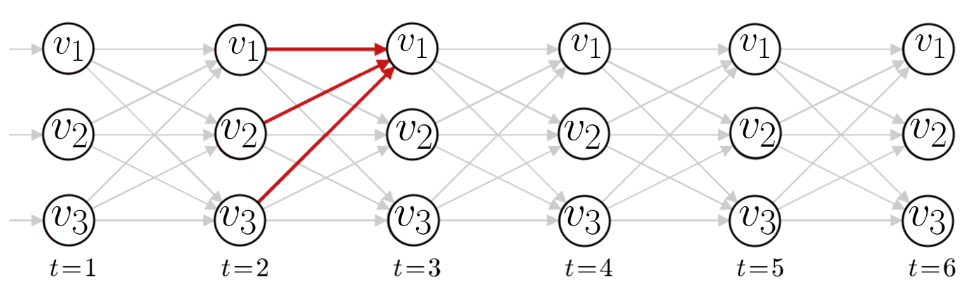 <!-- Initialization: $\alpha_1(i) = a_{0i} B(O_1|S_i)$ Recursion: $\alpha_{t+1}(i) = \sum_i \alpha_t(i) a_{ij} B(O_{t+1}|S_i)$ $$P(O|M) = \sum_{i=1}^M \alpha_{T}(i)$$ --> --- # Forward vs viterbi The only difference between Forward and Viterbi is you sum over all the possible paths instead of choosing the maximum: Viterbi recursion step: $ v_l(i) = e_l(x_i) \times max_k(v_k(i-1)a_{kl}) $ Forward algorithm recursion step: $ f_l(i) = e_l(x_i) \times \sum_{k}{f_k(i-1)a_{kl}} $ --- ### Forward-Backward algorithm: both directions Forward: Probability of the state for observations now and preceding Backward: Probability of the state for following observations Then: The two results combined give the distribution over states at any specific point, given the all observations. The probability of being in a given state at a particular point is $P(\pi_i = k|x) = \frac{f_k(i)b_k(i)}{P(x)}$ <!-- .element : class="fragment" data-fragment-index="1" --> Note: Because we are interested in comparison of states at each time point, we have to scale it. So we will calculate alpha-3F * beta3F / sum(alpha_iF*beta_iF). So when using this method, we also get some confidence values associated with our determination of the most likely state --- ## Learning problem Given observation sequence $O$, and general structure of HMM, determine HMM parameters that best fit the training data. ### Learning with annotated training data <!-- .element : class="fragment" data-fragment-index="1" --> If we had training data: A sequence of observations, with a known state sequence <!-- .element : class="fragment" data-fragment-index="1" --> We could just use maximum likelihood. We could compute: <!-- .element : class="fragment" data-fragment-index="1" --> - emission probability for each state <!-- .element : class="fragment" data-fragment-index="1" --> - transition probabilities for each state <!-- .element : class="fragment" data-fragment-index="1" --> - initial state probabilities <!-- .element : class="fragment" data-fragment-index="1" --> We have defined the model. <!-- .element : class="fragment" data-fragment-index="1" --> --- ## Estimating parameters for coin flips  --- ## Estimating parameters for coin flips  Emissions: $P(H|F), P(T|F), P(H|L), P(T|L)$ <!-- .element : class="fragment" data-fragment-index="1" --> Transitions: $P(F|F), P(F|L), P(L|F), P(L|L)$ <!-- .element : class="fragment" data-fragment-index="2" --> Problem: What if we don't have known state sequences? <!-- .element : class="fragment" data-fragment-index="3" --> Note: Consider a fully visible Markov model. This would easily allow us to compute the HMM parameters just by maximum likelihood estimation from the training data. For a real HMM, we cannot compute these counts directly from an observation sequence since we don’t know which path of states was taken through the machine for a given input. The Baum-Welch algorithm solves this by iteratively estimating the counts. We will start with an estimate for the transition and observation probabilities and then use these estimated probabilities and use the forward-backward procedure to determine the probability of the states at each observation. Then we can use that to determine better estimates of the transition and emission probabilities. --- ### Learning *without* annotated training data What algorithm have we seen that can be used to compute maximum likelihood estimates with incomplete data? * Input is only observations: $o_1, o_2, \ldots, o_T$ * Missing: The hidden state sequence --- ### Learning *without* annotated training data * Baum-Welch algorithm (EM algorithm) * Iteratively estimates the missing data and maximizes parameters * guaranteed to converge to a local optimum * not guaranteed to be a global optimum --- ### Baum-Welch Initialize parameters. E-step (expectation): Use forward-backward to estimate state probabilities M-stem (maximization): Adjust transition/emission probabilities in the model according to those estimated state probabilities. Iterate until convergence --- ## Advantages and limitations * Modularity: HMMs can be combined into larger HMMs * Transparency: Based on a state model making it interpretable * Prior knowledge: can be incorporated in the model * Need accurate, applicable, and sufficiently sized training sets of data * Model may not converge to a true optimum * Can be slow in comparison to other methods --- ## Applications 1. ChromHMM: chromatin state segmentation 2. HMMer: protein homology search 3. Universe-HMM: consensus interval sets --- ## ChromHMM > ChromHMM is a Java program for learning and characterizing chromatin states using a multivariate Hidden Markov Model that models the combinatorial and spatial patterns in data from multiple chromatin marks. --- ChromHMM Input is a binary matrix of chromatin mark presence/absence across genomic tiles. - Columns are chromatin marks - Rows are genomic tiles Example: ```console Cell chr1 Mark1 Mark2 Mark3 0 0 0 0 1 0 0 0 1 ``` --- ChromHMM output is a segmentation that divides the genome into chromatin states. Example 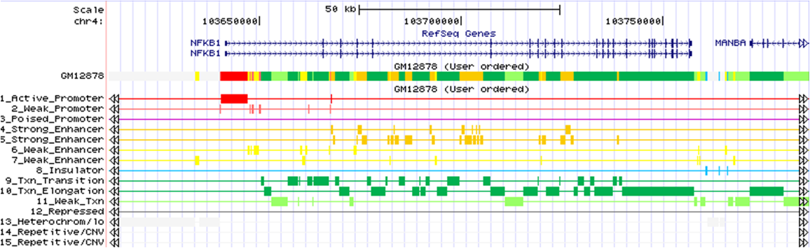 --- ## HMMEr > HMMER is a software package that provides tools for making probabilistic models of protein and DNA sequence domain families – called profile hidden Markov models, profile HMMs, or just profiles – and for using these profiles to annotate new sequences, to search sequence databases for additional homologs, and to make deep multiple sequence alignments --- HMMer input is a protein multiple-sequence alignment Example: 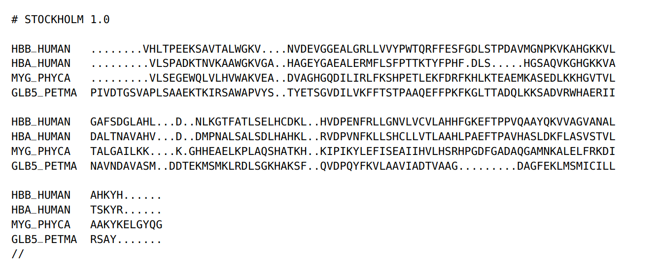 --- HMMer learns an HMM model from the input ``` hmmbuild globins4.hmm globins4.sto ``` 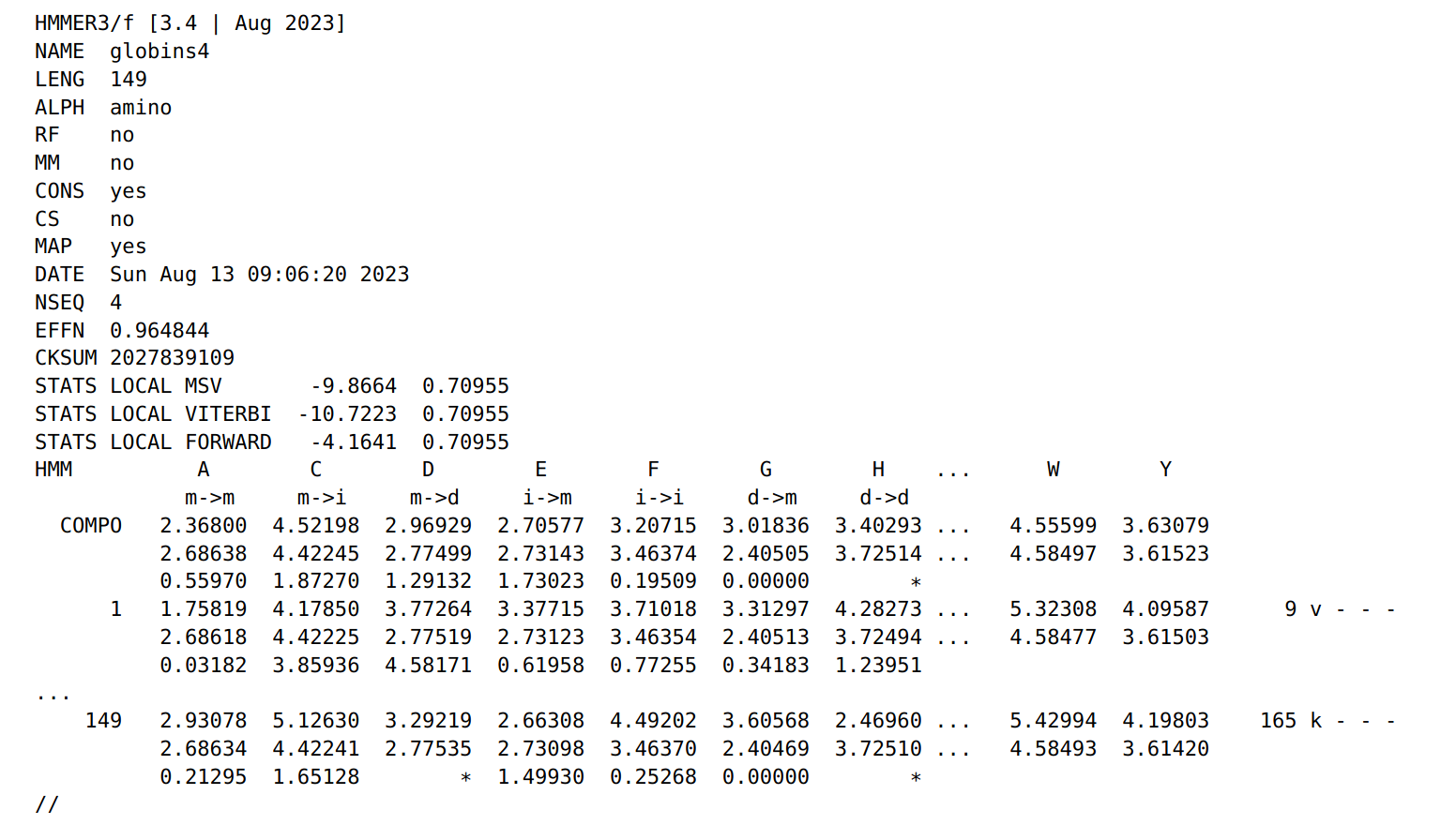 --- Trained HMMer models can be used to search sequence databases for other sequences that match the alignment. --- ## Consensus region set HMM > In our model, there are three observed sequences: the number of starts, overlaps, and ends at a given position. The hidden variable corresponds to the different parts of the flexible segment. We can tune transition probabilities, which can be chosen in a way that will prevent unnecessary segmentation, and emission matrix, which describes the relationship between observations and hidden states. --- Region set HMM input is a collection of region sets, which is transformed into counts of starts, overlap, and ends  <!-- .element style="background:white" --> Output is a unified segmentation, a consensus region set ---