## Sequence alignments  <!-- .element height="80%" width="80%" --> --- ## Why might we want to align sequences? * Detect orthologs * Identify functional elements * Understand neo-functionalization of genes * Identify variants in a population * ... --- ## All species share common ancestry  <!-- .element height="80%" width="80%" --> <small>Source : [Wikipedia](https://commons.wikimedia.org/wiki/File:Phylogenetic_tree.svg)</small> Note: A phylogenetic tree of living things, based on ribosomal RNA data and proposed by Carl Woese in 1977, showing the separation of bacteria, archaea, and eukaryotes. Trees constructed with other genes are generally similar, although they may place some early-branching groups very differently, thanks to long branch attraction. The exact relationships of the three domains are still being debated, as is the position of the root of the tree. It has also been suggested that due to lateral gene transfer, a tree may not be the best representation of the genetic relationships of all organisms. For instance some genetic evidence suggests that eukaryotes evolved from the union of some bacteria and archaea (one becoming an organelle and the other the main cell). --- ## Genome-wide alignments reveal orthologous segments 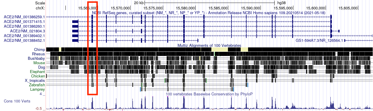 Note: This signal can be used to determine orthologous genes in other species --- ## Comparative genomics reveals functional elements  --- ## What makes us human? 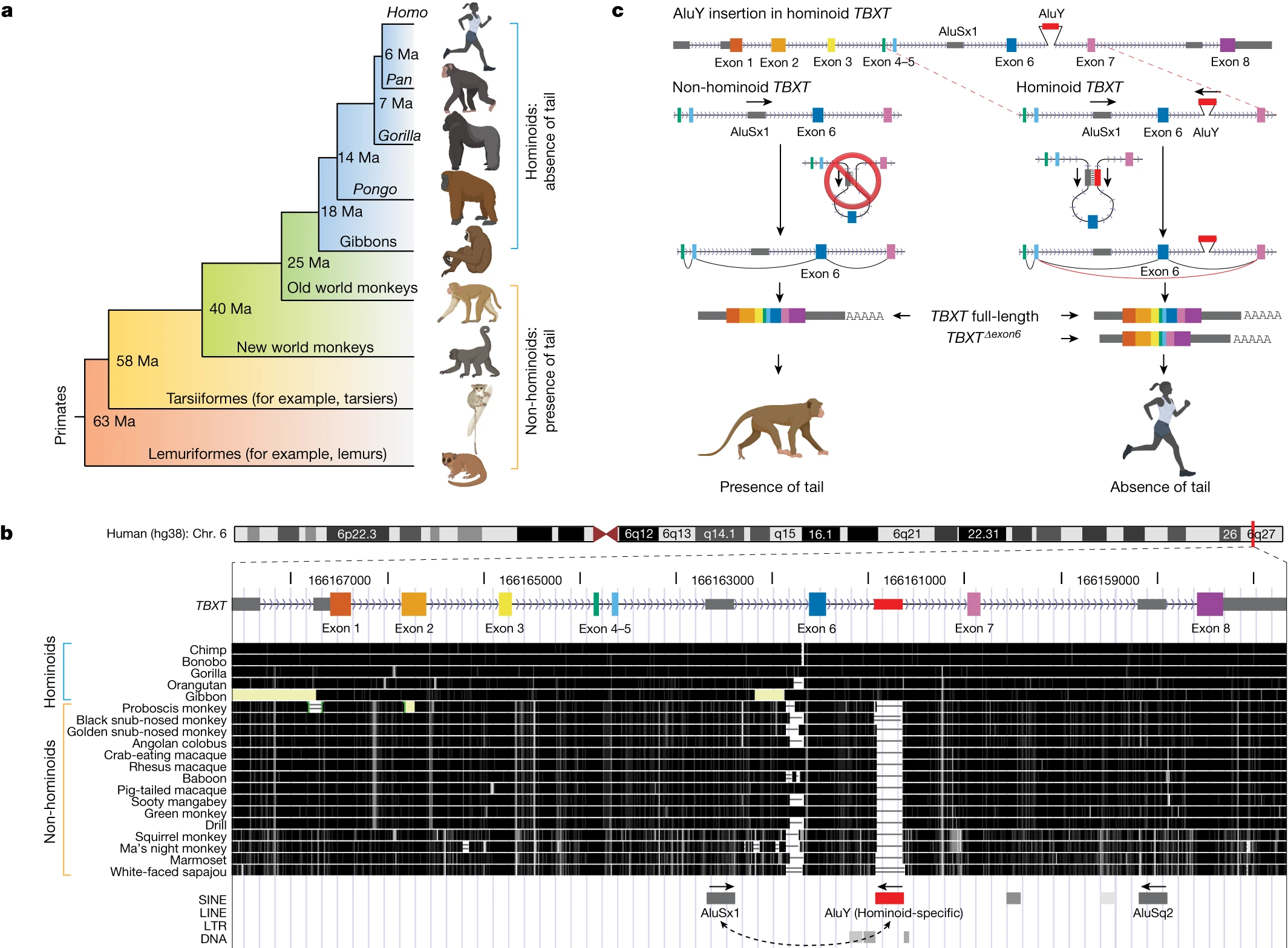 <!-- .element height="80%" width="80%" --> Source: PMC10901737 Note: a, Tail phenotypes across the primate phylogenetic tree. Ma, millions of years ago. b, UCSC Genome browser view51 of the conservation score through multi-species alignment at the TBXT locus across primate genomes. Exon numbering of human TBXT follows a conventional order across species without including the 5′ untranslated region exon. The hominoid-specific AluY element is highlighted in red. LINE, long interspersed nuclear element; LTR, long terminal repeat; SINE, short interspersed nuclear element. c, Schematic of the proposed mechanism of tail-loss evolution in hominoids. --- ## How do we actually align two sequences? 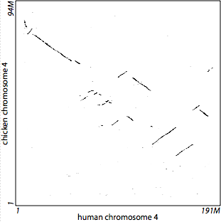 --- ## Outline 1. Introduction to sequence alignment 2. Dynamic programming for sequence alignments 3. Exact matching 4. Database search 5. Short-read alignment --- ## Genomes change over time  <!-- .element height="30%" width="30%" --> --- ## Goal of genome alignment  <!-- .element height="30%" width="30%" --> --- ## Goals of genome alignment  <!-- .element height="80%" width="80%" --> --- ## Formalizing the problem  <!-- .element height="50%" width="50%" --> * Define a set of evolutionary operations * Assumption : Symmetric operations * Define optimality criterion * min (\# of operations) $\ldots$ * Design algorithm that achieves optimality * Assumptions influence performance Note: The evolutionary operation we are going to consider are insertion, deletion and substitutions. Minimum cost of operations can be another optimality criterion. When comparing human and mouse, we do not try to infer the bases in the ancestor of the human and mouse, but we reverse the time direction of a branch and then think of operation that might have occurred. Also remember that it is Impossible to infer exact series of operations (Occams razor). We want to design an algorithm that achieves optimality or at least can approximate it. If we can provide concrete bounds on that approximation then that is the ideal case. --- ## Formalizing the problem  <!-- .element height="50%" width="50%" --> * Define a set of evolutionary operations * Assumption : Symmetric operations * Define optimality criterion * min (\# of operations) $\ldots$ * Design algorithm that achieves optimality * Assumptions influence performance --- ## Algorithmic complexity Big-O notation: upper bound on complexity  <!-- .element height="50%" width="50%" --> <small>Recommended reading: Chapter 3, "Growth of functions" in [The Big Book](https://search.lib.virginia.edu/?mode=basic&q=keyword:+{Introduction+to+Algorithms}&pool=uva_library)</small> Note: We will often want to talk about how long does an algorithm take to complete given an input of size $n$?, or How much space does an algorithm need to complete given an input of size $n$. To the right of n0, the value of the function is always lower than g(n) by a constant factor. Upper bound on coplexity signifies the worst-case performance of the algorithm, and makes it easy to compare different algorithms because the notation tells clearly how the algorithm scales when input size increases. Typically we are tying to see if we can change g(n), but in some cases reducing the factor can lead to large gains. g(n) is often referred to as the order of growth. --- ## Order of growth 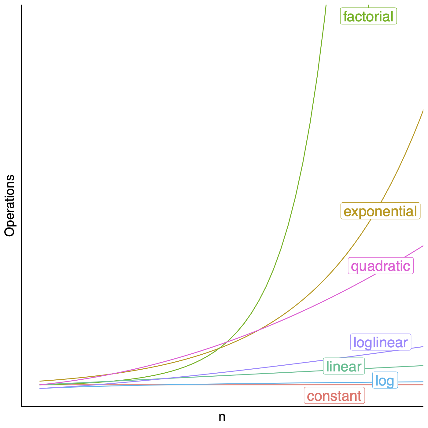 <!-- .element height="50%" width="50%" --> Note: Constant runtime is represented by O(1), linear growth is O(n), logarithmic growth is O(log n), log-linear growth is O(n log n), quadratic growth is O(n^2), exponential growth is O(2^n), factorial growth is O(n!). --- ## Longest common substring Given two possibly related strings $x$ and $y$, what is the longest common substring (no gaps)? ```text x : TCACCTGACCTCCAGGC y : TCATGACCGCCATGGC ``` ```text x : TCACCTGACCTCCAGGC |||xxxxxx|xxxx|x y : TCATGACCGCCATGGC ``` <!-- .element: class="fragment" data-fragment-index="1" --> --- ## Longest common substring Given two possibly related strings $x$ and $y$, what is the longest common substring (no gaps)? ```text x : TCACCTGACCTCCAGGC y : TCATGACCGCCATGGC ``` ```text x : TCACCTGACCTCCAGGC xxxxxxx|xx|xx||| y : TCATGACCGCCATGGC ``` --- ## Longest common substring Given two possibly related strings $x$ and $y$, what is the longest common substring (no gaps)? ```text x : TCACCTGACCTCCAGGC y : TCATGACCGCCATGGC ``` ```text x : TCACCTGACCTCCAGGC ||||| y : TCATGACCGCCATGGC ``` --- ## Longest common substring Given two possibly related string $x$ and $y$, what is the longest common substring (no gaps)? ```python max_run_length = 0 for i in range(0, len(x)): maxr = longest_run(x, i, min(len(x), i+len(y)), y, 0, min(len(y), len(x)-i)) if maxr > max_run_length: max_run_length = maxr for i in range(0, len(y)): maxr = longest_run(x, 0, len(y)-i, y, i, len(y)) if maxr > max_run_length: max_run_length = maxr print(max_run_length) ``` Note: So this requires comparing all letters at each offset, and it would be quadratic in the length of the shorter sequence. --- ## Longest common subsequence * A subsequence is a sequence that appears in the same relative order, but not necessarily contiguous * abc, abg, bdf, $\ldots$ are subsequences of abcdefg * Given two possibly related string $x$ and $y$, what is the longest common subsequence? ```text x : TCACCTGACCTCCAGGC y : TCATGACCGCCATGGC ``` ```text x : TCACCTGACCTCCA-GGC ||| |||||x||| ||| y : TCA--TGACCGCCATGGC ``` Note: It differs from the longest common substring problem: unlike substrings, subsequences are not required to occupy consecutive positions within the original sequences. This problem is related to the edit distance, minimum number of operations required to transform one string into the other. This is getting closer to the problem that we want to tackle for alignment of sequences. For now let's keep this simplistic assumption that all mismatches and gaps are equally penalized, but remember that this is simplistic. We make these sort of simplistic assumptions while developing algorithms, similar to using brute-force to see if a problem is tractable. --- ## Brute-force approach * $|x|=n,\ |y|=m, \ n > m$ * Longest alignment : $n+m$ entries * Alignment is a gap-placement algorithm * ${n+m \choose n}$ ways of placing gaps in $y \approx 2^{m+n}$ 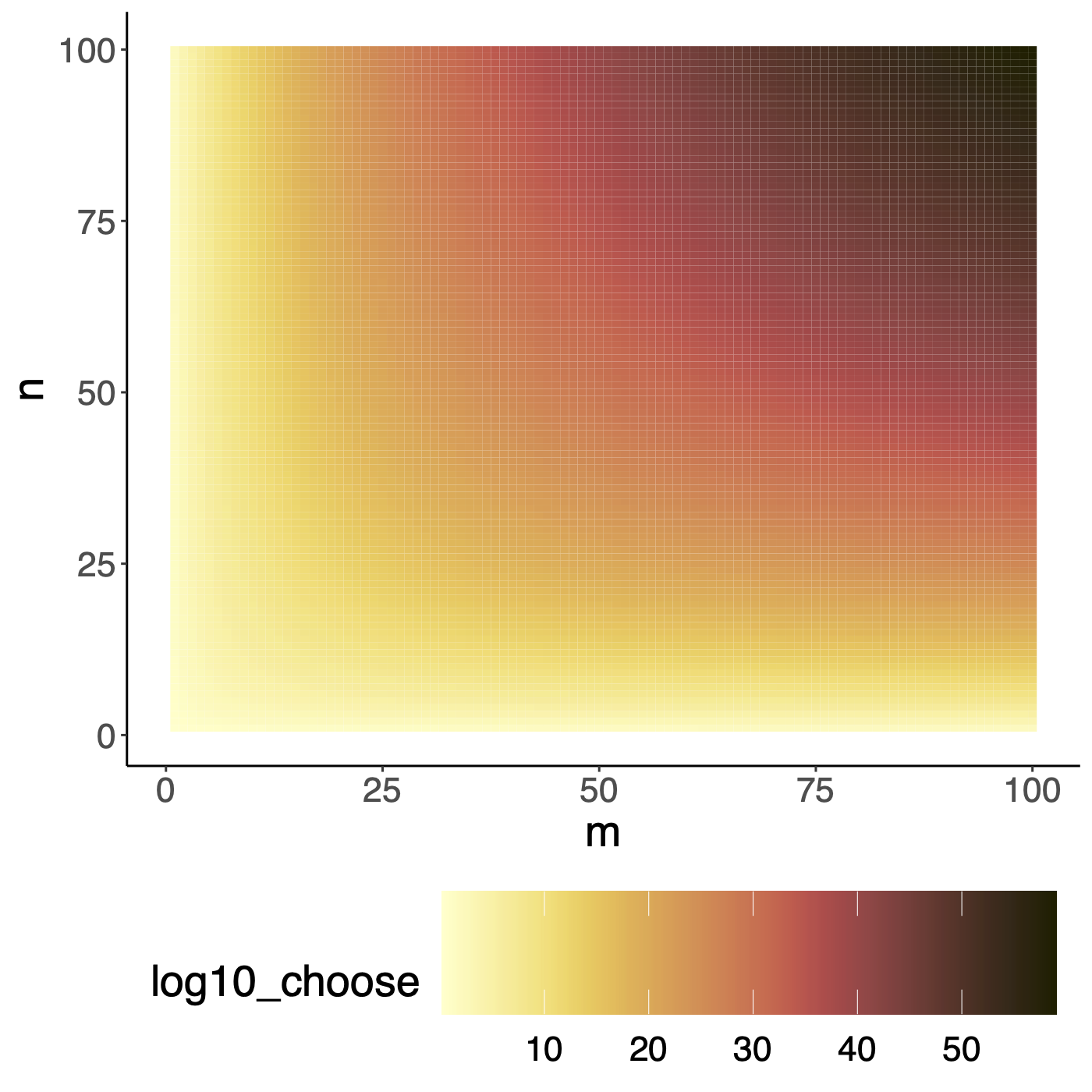 <!-- .element height="30%" width="30%" --> Note: Enumerating and scoring them is not an option. Need a polynomial algorithm to find the best alignment amongst exponential number of alignments. Whenever you want to explore an exponential search space in polynomial time, a technique you should think of is dynamic programming. --- ## Dynamic Programming in theory * Hallmarks of dynamic programming * Optimal substructure * Overlapping sub-problems <!-- * For optimization problems * Optimal choice is made locally * Score is added through the search space * Traceback common, find optimal path based on the individual choices --> Note: Optimal substructure: Optimal solution to problems contains optimal solution to sub-problems. Overlapping sub-problems : Limited number of distinct sub-problems, repeated many times. Another set of algorithms that operate on problems with optimal substructure are called greedy algorithms. Faster, easier to set up, but often you are not guaranteeing optimal solution, and when looking at subproblems, you are never revising your solution. An example is the Dijkstra’s shortest path algorithm --- ## Sequence alignments: Optimal substructure Let $X=[x_1,\...,x_m]$ and $Y=[y_1,\...,y_n]$ be sequences, and $Z=[z_1,\...,z_k]$ be a LCS of $X$ and $Y$. 1. If $x_m = y_n$, then $z_k = x_m = y_n$ and $Z_{k-1}$ is a LCS of $X_{m-1}$ and $Y_{n-1}$. 2. If $x_m \neq y_n$, then $z_k \neq x_m$ implies $Z$ is a LCS of $X_{m-1}$ and $Y$. 3. If $x_m \neq y_n$, then $z_k \neq y_n$ implies $Z$ is a LCS of $X$ and $Y_{n-1}$. --- ## Sequence alignments: Overlapping subproblems  <!-- .element height="70%" width="70%" --> --- ## Sequence alignment: optimal substructure Define $OPT(i,j)$ = min cost of aligning prefix strings $x_1, x_2, \ldots, x_i$ and $y_1, y_2, \ldots, y_j$ * Case1. $OPT(i,j)$ matches $x_i - y_j$ * match or mismatch for $x_i – y_j$ + $OPT(x_{i-1}, y_{j-1})$ * Case2a. $OPT(i,j)$ leaves $x_i$ unmatched * gap for $x_i$ + $OPT(x_{i-1}, y_j)$ * Case 2b. $OPT(i,j)$ leaves $y_j$ unmatches * gap for $y_j$ + $OPT(x_i, y_{j-1})$ Note: Optimal solution to problems contains optimal solution to sub-problems, as defined here, so sequence alignment certainly has optimal substructure --- ## So how does this look?  --- ## Exploring the search space  --- ## Exploring the search space  --- ## Dynamic Programming * Create a large table indexed by $(i,j)$ * Decide on the recursion formula * Decide on optimal traversal order * Compute each sub-alignment once * Remember the choices Note: Use memoization (storing the results of expensive function calls and returning the cached result) for sub-problem if they are reused. If the subproblems are not reused, then maybe DP is not the right choice as an algorithm. Computation order matters, and most times bottom up will work though it is not obvious a lot of the times. Once you have the set up, then start filling the table, find the optimal score. Traceback to find the optimal solution. --- ## Computing alignment recursively * Local update rules, only look at neighboring cells * Computing the score of a cell from smaller neighbors `$$M(i,j) = max \left\{ \begin{array}{1} M(i-1,j) - gap\\ M(i-1, j-1) + score\\ M(i, j-1) -gap \end{array} \right\} $$` * Compute scores for prefixes of increasing length$\ \ \ \ \ \ $ --- ## Example  <!-- .element height="40%" width="40%" --> --- ## Example  <!-- .element height="40%" width="40%" --> --- ## Example  <!-- .element height="40%" width="40%" --> --- ## Example  <!-- .element height="40%" width="40%" --> --- ## Example  <!-- .element height="40%" width="40%" --> --- ## Returning an optimal path  <!-- .element height="40%" width="40%" --> --- ## Returning an optimal path  <!-- .element height="40%" width="40%" --> --- ## Returning an optimal path  <!-- .element height="40%" width="40%" --> --- ## Returning an optimal path  <!-- .element height="40%" width="40%" --> --- ## Returning an optimal path  <!-- .element height="40%" width="40%" --> --- ## Returning an optimal path  <!-- .element height="40%" width="40%" --> --- ## Returning an optimal path  <!-- .element height="40%" width="40%" --> --- ## Returning an optimal path  <!-- .element height="40%" width="40%" --> --- ## Returning an optimal path  <!-- .element height="40%" width="40%" --> --- ## Returning an optimal path  <!-- .element height="40%" width="40%" --> --- ## Returning an alternate optimal path  <!-- .element height="40%" width="40%" --> --- ## Sequence alignment * Allow gaps * Insertions and deletions * unit cost for each character deleted or inserted * Varying penalties for edit operations * Transitions vs. Transversions * Affine gap * Frame-aware gap Note: Time needed O(mn) and space needed O(mn) --- ## Insight : A gap changes the diagonal  <!-- .element height="40%" width="40%" --> --- ## Linear-time bound DP  <!-- .element height="40%" width="40%" --> --- ## Linear-space bound DP  <!-- .element height="40%" width="40%" --> --- ## Linear-space bound DP  <!-- .element height="40%" width="40%" --> --- ## Linear-space bound DP  <!-- .element height="40%" width="40%" --> --- ## Linear-space bound DP * Best score can be computed in linear space * use just one column/row * Traceback? * Using a divide and conquer approach * A [description with pseudocode](https://www.cs.cmu.edu/~ckingsf/bioinfo-lectures/linspace.pdf) from Carl Kingsford at CMU * Manuscript from [Myers and Miller](http://www.cs.ucf.edu/courses/cap5510/fall2009/SeqAlign/Linear_Space_Alignment.pdf) --- ## Local alignments A local alignment of string $s$ and $t$ is an alignment of a substring of $s$ with a substring of $t$ * Why local alignments? * Small domains of a gene may be only conserved portions * Looking for a small gene in a large chromosome * Large segments often undergo rearragments --- ## Local alignment vs Global alignment  <!-- .element height="50%" width="50%" --> --- ## Global Alignment (Needleman-Wunsch algorithm) **Initialization:** $F(0,0) = 0, F(i,0) = -gap \times i, F(0, j) = -gap \times j$ **Iteration:** `$$F(i,j) = max \left\{ \begin{array}{1} F(i-1,j) - gap\\ F(i-1, j-1) + score\\ F(i, j-1) -gap \end{array} \right\} $$` **Termination:** Bottom right --- ## Local alignment (Smith-Waterman algorithm) **Initialization:** $F(i,0) = F(0,j) = 0$ **Iteration:** `$$F(i,j) = max \left\{ \begin{array}{1} 0\\ F(i-1,j) - gap\\ F(i-1, j-1) + score\\ F(i, j-1) -gap \end{array} \right\} $$` **Termination:** Anywhere --- ## More variations * Semi-global alignment * At least one of the sequences to the end * Different gap penalties * Affine gap penalties * Length mod 3 penalties for protein coding regions Recurrence equation with modifications can accomodate these variations --- ## Dynamic Programming * https://github.com/uvacobi/sequence_alignment * Implement local alignment of two sequences that can use affine gap penalties * Skeleton code is provided in python * Simple test cases are also provided * Clone the repo, implement the `smith_waterman` function in `align_sequences.py` * You can test your work by running `python3 testdriver` --- ## Linear time exact matching * gene in chromosome (local alignment is expensive) * Karp-Rabin algorithm * Insight : if $|\sum|= d$, a string represents a number in base $d$ * AGCT = 0123 --- ## Karp-Rabin algorithm Insight: Interpret string as numbers for fast comparisons  --- ## Karp-Rabin algorithm Compute next number based on the previous one  * Shift middle digits of the number to the left * Remove the higher order bit * Add the low order bit --- ## Karp-Rabin algorithm * Reduce the number of comparisons using hashing * Mapping keys $k$ from large universe $U$ (of string/numbers) into a smaller space $[1..m]$ * Many hash functions possible with theoretical and practical properties * Reproducibility: $x=y \rightarrow h(x) = h(y)$ * Uniform output distribution: $x \ne y \rightarrow P(h(x) = h(y)) = 1/m$ * Worst case runtime $O(mn)$ Note: if every position is a match or false-positive --- ## Karp-Rabin algorithm 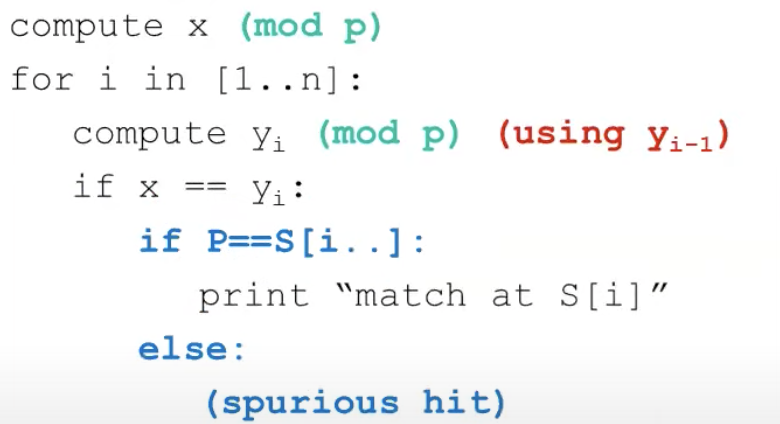 <!-- .element height="50%" width="50%" --> --- ## BLAST and inexact matching * Sequence alignment * Sequences have some common ancestry * Find optimal alignment between two sequences * Evolutionary interpretation: min # events, ... * Sequence database search * Given a query and target sequences: which sequences are related to the query * Individual alignments need not be perfect * Most sequences are completely unrelated to query Note: Basic Local Alignment Search Tool --- ## BLAST * Exploit the nature of the problem * Prescreen sequences for common stretches * Preprocess the database if it is offline * Key insights * Semi-numerical string matching like Karp-Rabin * Neighborhood search --- ## Blast algorithm overview  <!-- .element height="70%" width="70%" --> <small>[The Statistics of Sequence Similarity Scores](https://www.ncbi.nlm.nih.gov/BLAST/tutorial/Altschul-1.html)</small> Note: * Split query into overlapping words of length W. * Find neighborhood words for each word until threshold T. * Look in table where these neighbor words occur: seeds S. * Extend seeds S until score drops off under X. * Report significance and alignment of each match --- ## Why does BLAST work? * Pigeonhole principle * if $n$ items are put into $m$ containers, with $n>m$, then at least one container must contain more than one item * Applying to alignments * Two sequences, each 9 amino-acids, with 7 identities * 3 amino-acids perfectly conserved --- ## Extensions to the basic algorithm * Filtering : Low complexity regions * Two hit BLAST * Two smaller W-mers more likely than a long one * Non-consecutive k-mers * No reason to use only consecutive symbols * RGIKW $\rightarrow$ R\*IK\*, RG\*\*W, $\ldots$ * How to choose positions for *: * Random * Learn from data --- ## Aligning two strings  <!-- .element height="40%" width="40%" --> --- ## Querying a database  <!-- .element height="70%" width="70%" --> ---