## Genome assembly 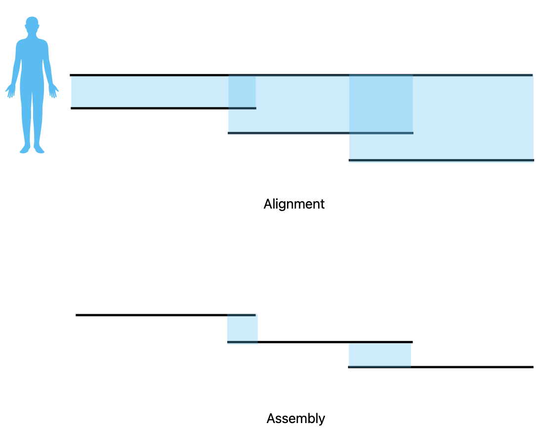 <!-- .element height="80%" width="80%" --> <small>Acknowledgement: Some slides borrowed with permission from Dr. Ben Langmead, JHU</small> --- ## Shotgun sequencing and genome assembly <iframe width="659" height="371" src="https://www.youtube.com/embed/pfgnrOOwqSU" title="YouTube video player" frameborder="0" allow="accelerometer; autoplay; clipboard-write; encrypted-media; gyroscope; picture-in-picture" allowfullscreen></iframe> <a href="https://www.youtube.com/embed/pfgnrOOwqSU" class="small">HHMI</a> Note: Shotgun sequencing requires multiple copies of the genome, which are effectively blown up into millions of small fragments. Each fragment is then sequenced. The small fragments are assembled using an immense amount of computer power to match overlapping sections. The drawback of this method comes when dealing with repeat sequences. Often there is no way of knowing how long the repeat sequence is. Or in which of the many different possible positions the fragments overlap. Even the incredibly powerful software used to shotgun sequence the human genome couldn't cope with this. So Celera, the private company which relied on this approach, had to use the public data to fill in the gaps left by the repeats. --- ## Shotgun sequencing  --- ## Shotgun sequencing  --- ## Shotgun sequencing  --- ## Genome assembly  --- ## Genome assembly  --- 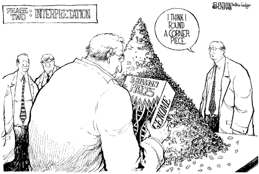 <small>Human Genome cartoons, Slate magazine, US</small> --- ## Genome assembly  --- ## Coverage  --- ## Gaps  --- ## Statistics * Parameters * $G$ = genome length in nucleotides * $L$ = read length in nucleotides * $N$ = number of reads sequenced * Coverage $a$ = $NL/G$ --- ## Statistics * Assume reads are distributed uniformly through the genome. * The probability that one of the $N$ reads starts at any specific nucleotide is $N/G$.  --- ## Statistics * The probability that one of the $N$ reads starts at any specific nucleotide is $N/G$. * Expected # of reads starting in interval $I$ of length $L$ is $NG/L = a$ * We can assume a poisson distribution * $\lambda$ events in a given interval * probability of k events = ${\frac {\lambda ^{k}e^{-\lambda }}{k!}}$ * $p$ = $P$(no read starts in $I$) = $e^{-a}$ * $q$ = $P$(at least one read starts in $I$) = $1 - e^{-a}$ Note: The other option is a binomial distribution when p=(1 - N/G)^L, but poisson is more accurate in casee when its likely that multiple reads start at the same position. --- ## Statistics How much of the genome was sequenced? * Position $x$ is in a gap if no read starts in $[x − L + 1, x]$ * We showed this has probability $p = e^{−a}$ * Estimates * Nucleotides in gaps = $pG$ = $e^{-a}G$ * Nucleotides in contigs = $qG$ = $(1 - e^{-a})G$ * To have 99% genome in contigs and 1% in gaps: * $p = e^{−a} = 0.01$ * $a \approx 4.6$ * So, sequence 13.8 billion nucleotides, and you will still miss 30 million positions in the genome --- ## Genome assembly  --- ## Pairwise overlaps  <!-- .element width="70%" height="70%" --> Note: Even in this case, why could there be differences? 1. sequencing errors, 2. ploidy (humans have 2 copies of each chromosome, and those copies can be different). Real assemblers have to account for ploidy, but we are going to ignore it to simplify issues in this lecture. --- ## More is better?  <!-- .element width="70%" height="70%" --> Note: If we assume that sequencing of reads is random, then as more reads are sequenced, more start points for the reads and hence larger overlaps are reasonable. --- ## Two approaches to assembly  <!-- .element width="70%" height="70%" --> --- ## Overlap Layout Consensus  <!-- .element width="70%" height="70%" --> Notes: Examples of such assemblers include SGA, Fermi --- ## Overlap Overlap : Suffix of a read is similar to the prefix of another read  <!-- .element width="50%" height="50%" --> --- ## Overlap Overlap : Suffix of a read is similar to the prefix of another read  <!-- .element width="50%" height="50%" --> Note: We can represent such an overlap with a directed graph, where directed edges connect overlapping nodes (reads). The suffix of source is similar to the prefix of sink. Effectively, we want to do this for all pair of reads to build our overlap graph. --- ## Overlap graph Overlap graph can contain cycles. A cycle is a path beginning and ending at the same vertex.  Note: This is possible if the sequenced genome is circular (bacterial genomes, mtDNA). And in the case of repeats. --- ## An example digraph <small>GCATTATATATTGCGCGTACGGCGCCGCTACA, read-length : 7, minimum overlap : 3</small><br>  <!-- .element width="40%" height="40%" --> Note: In order to keep the presentation uncluttered, we are not showing the treatment of the reverse complements --- ## Overlap Layout Consensus 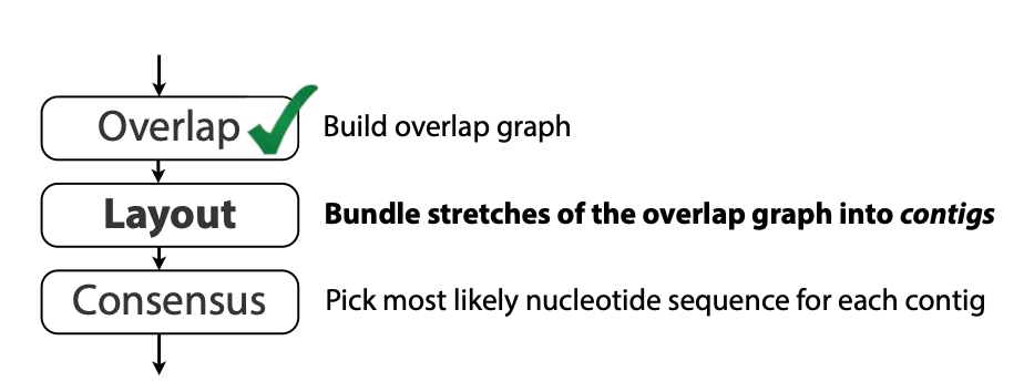 <!-- .element width="90%" height="90%" --> --- ## Layout The overlap graph is big and messy. 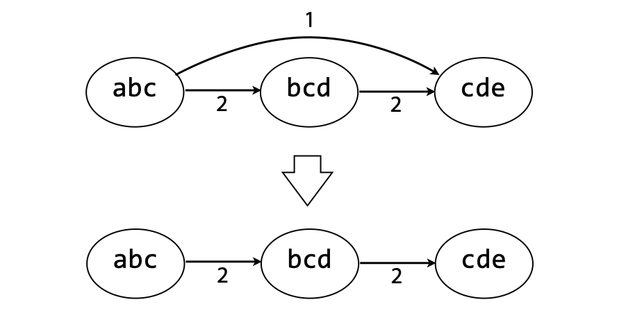 <!-- .element width="80%" height="80%" --> Note: But the picture gets clearer after removing transitively-inferrible edges. --- ## Layout Remove transitively-inferrible edges<br>  <!-- .element width="40%" height="40%" --> --- ## Layout Removing edges that skip one node.<br>  <!-- .element width="40%" height="40%" --> --- ## Layout Removing edges that skip two nodes.<br>  <!-- .element width="40%" height="40%" --> --- ## Layout Removing edges that skip three nodes.<br>  <!-- .element width="40%" height="40%" --> --- ## Layout 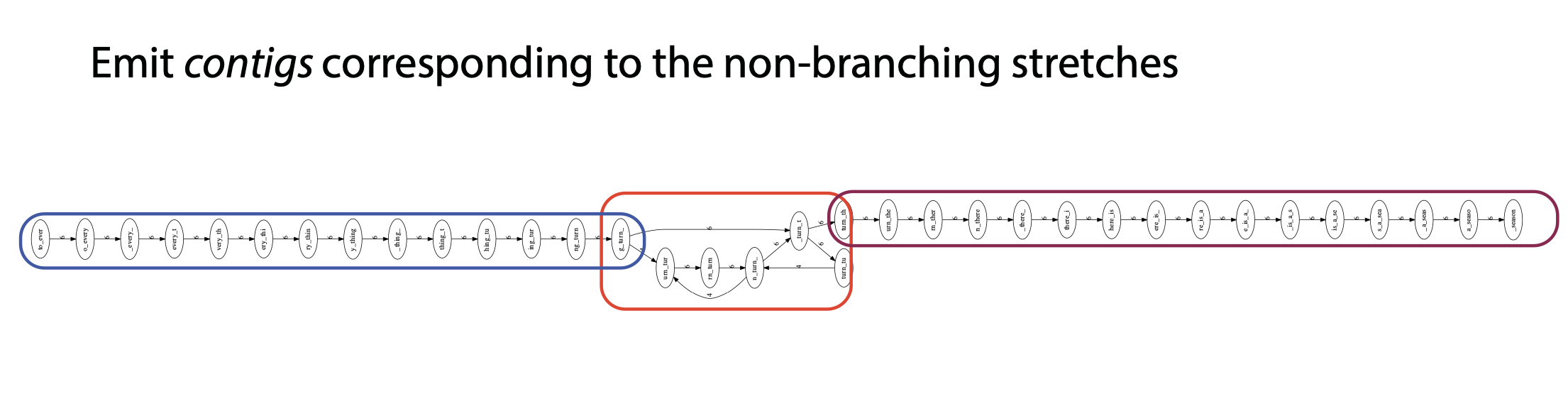 <!-- .element width="95%" height="95%" --> Note: Can someone tell me what could be the cause of the branches? --- ## Repeats 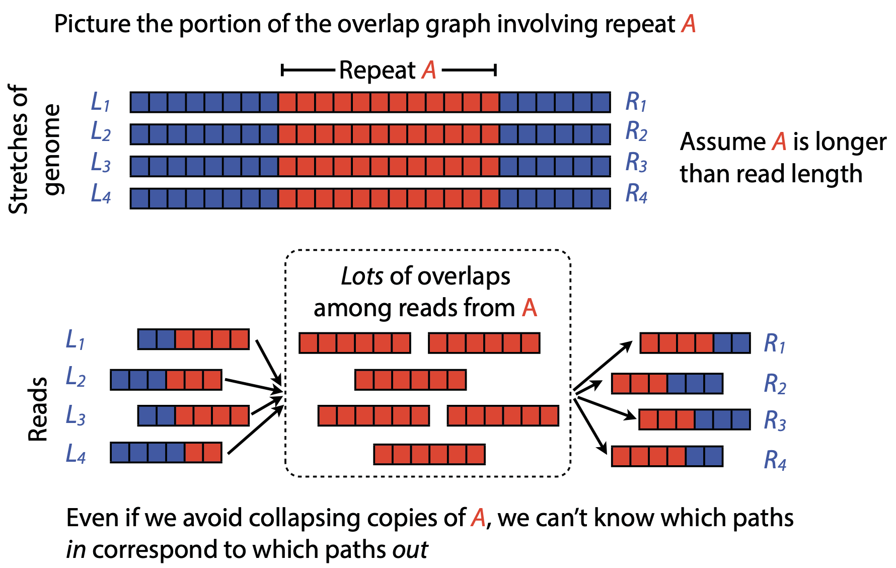 <!-- .element width="95%" height="95%" --> Note: This is also why longer reads are extremely helpful with genome assembly. For some of the assemblies we have recently done for humans, we can assemble close to complete chromosomes after we use some additional information from conformation capture experiments --- ## Layout In practice, layout step also has to deal with spurious subgraphs, e.g. because of sequencing error  <!-- .element width="95%" height="95%" --> Note: Mismatch could be due to sequencing error or repeat. Since the path through b ends abruptly we might conclude it’s an error and prune b. --- ## Overlap Layout Consensus  <!-- .element width="90%" height="90%" --> --- ## Consensus  <!-- .element width="95%" height="95%" --> --- ## Consensus  <!-- .element width="70%" height="70%" --> Note: At each position, ask: what nucleotide (and/or gap) is here? Complications: (a) sequencing error, (b) ploidy. --- ## Overlap Layout Consensus  <!-- .element width="70%" height="70%" --> Note: Main drawback of OLC is Building overlap graph can be slow, specially for NGS data where we have billions of reads. Building a consensus requires incorporation of heuristics in order to determine the number of repeat units for example. --- ## Two approaches to short read assembly  <!-- .element width="80%" height="80%" --> --- ## De Bruijn graph  --- ## De Bruijn graph  A walk crossing each edge exactly once gives a reconstruction of the genome. This is an Eulerian walk. --- ## Eulerian walks * Node is balanced if indegree equals outdegree * Node is semi-balanced if indegree differs from outdegree by 1 * Graph is connected if each node can be reached by some other node * Eulerian walk visits each edge exactly once * Not all graphs have Eulerian walks. A directed, connected graph is Eulerian if and only if it has at most 2 semi-balanced nodes and all other nodes are balanced <!-- .element class="fragment" data-fragment-index="1" --> --- ## Eulerian walks  AA and BA are semi-balanced, AB and BB are balanced --- ## Constructing De Bruijn graph * Pick a substring length $k$ * For each *k* mer in the string * Split *k* mer into left and right *k-1* mers * Add *k-1* mers as nodes to de Bruijn graph * Add edge from left *k-1* mer to right *k-1* mer $k$ is typically chosen to be odd, so a *k*mer is not it's own reverse complement. Example: TCGCGA Note: When the first half of the kmer is reverse complement of the second half, then we have a situation where the kmer is its own reverse complement. --- ## Constructing De Bruijn graph <small>Sequence : GTGCGCTAATCGGAGACGAATTTAAGACAC</small><br>  <!-- .element width="30%" height="30%" --> --- ## Constructing De Bruijn graph <small>Sequence : GTGCGC<span style="color:red">TAATCGGAGACGAATTTAAG</span>ACAC<span style="color:red">TAATCGGAGACGAATTTAAG</span></small><br>  <!-- .element width="37%" height="37%" --> Note: There are two things to appreciate here. Node for k-1-mer from left end is semi-balanced with one more outgoing edge than incoming. Node for k-1-mer at right end is semi-balanced with one more incoming than outgoing. The only exception here is that left- and right-most k-1-mers are equal. Other nodes are balanced since # times k-1-mer occurs as a left k-1-mer = # times it occurs as a right k-1-mer. So the graph produced is Eulerian. Addition of duplicates does not increase the number of nodes significantly. Edges increase, but we can replace edges with edge weights. --- ## De Bruijn graph For a Eulerian graph, Eulerian walk can be found in $O(|E|)$ time. Note: |E| is the number of edges. Convert graph into one with Eulerian cycle (add an edge to make all nodes balanced). We want to be able to traverse the whole graph. We then start from a node and we are going to keep visiting unvisited edges till we get back to v. It is not possible to get stuck at any vertex other than v, because indegree and outdegree of every vertex must be same, when the trail enters another vertex w there must be an unused edge leaving w. The tour formed in this way is a closed tour, but may not cover all the vertices and edges of the initial graph. As long as there exists a vertex u that belongs to the current tour, but that has adjacent edges not part of the tour, start another trail from u, following unused edges until returning to u, and join the tour formed in this way to the previous tour. --- ## De Bruijn graph <small>Sequence : GTGCGCTAATCGGAGACGAATTTAAGACAC</small><br>  <!-- .element width="30%" height="30%" --> --- ## De Bruijn graph <small>Sequence : GTGCGC<span style="color:red">TAATCGGAGACGAATTTAAG</span>ACAC<span style="color:red">TAATCGGAGACGAATTTAAG</span></small><br>  <!-- .element width="37%" height="37%" --> --- ## De Bruijn graph  <!-- .element width="30%" height="30%" --> Walk 1: ZA→AB→BE→EF→FA→AB→BC→CD→DA→AB→BY Walk 2: ZA→AB→BC→CD→DA→AB→BE→EF→FA→AB→BY --- ## De Bruijn graph * Repeats still cause misassembles * Real datasets have sequencing errors * Gaps in coverage lead to disconnected or non-Eulerian graph * Difference in coverage can make graph non-Eulerian Note: Casting assembly as Eulerian walk is appealing, but not practical. Uneven coverage, sequencing errors, etc make graph non-Eulerian. Even if graph were Eulerian, repeats yield many possible walks --- ## Graph Topology based error-correction  --- ## *k*mer based error correction  <small>[PMC6311904](https://www.ncbi.nlm.nih.gov/pmc/articles/PMC6311904/)</small> Note: Frequency distribution of both error-free and error-containing k-mers for a NGS data set. The frequency distribution of erroneous k-mers is represented by the dash orange line, while the distribution of the correct ones is shown as the dash sky-blue line. The solid black line is the distribution of all the k-mers. The α-labeled area is the proportion of correct k-mers having frequency less than f0, while the β-labeled area is the proportion of erroneous k-mers having frequency greater than f0 ---