reveal.js

## Network analysis
![networks](images/networks/title.png)

---

## Outline

* Introduction to networks
    * Representations
* Global/Local network properties
    * Emergent properties
    * Centrality
* Guilt by association
    * Direct methods
    * Module-assisted

Note: Networks are everywhere in the world, including social networks, collaboration networks, transportation networks, computer networks and biological networks.

---

## Examples of biological networks

Regulatory networks

![example](images/networks/regulatory.png)

<small>Source: Modified from PMC6302376</small>

Note: directed: who regulates what, signed: activation or repression, weighted: how much do I regulate.

---

## Examples of biological networks

Protein-protein interaction network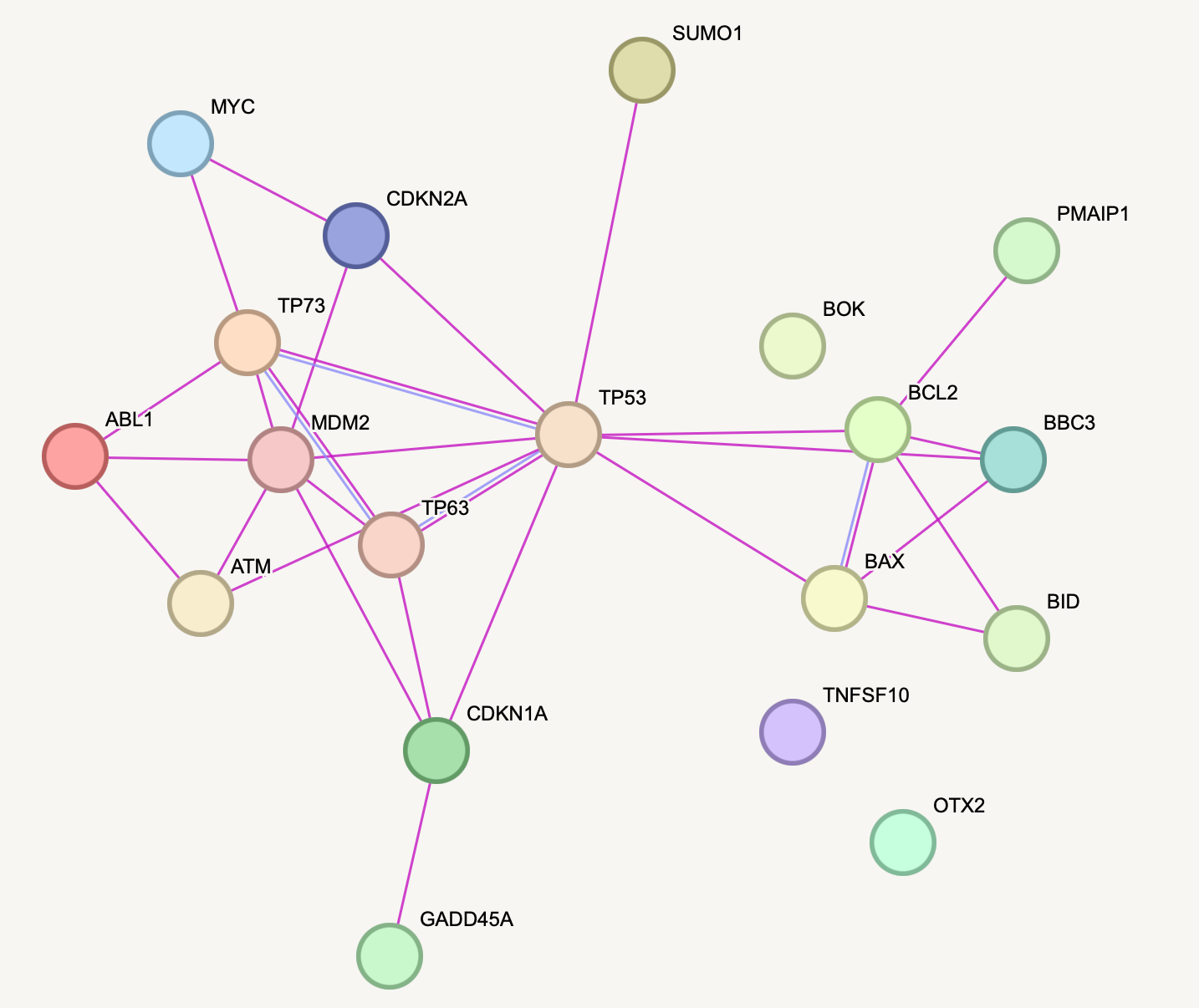 
![example](images/networks/ppi.png)

Notes: STRING subnetwork of TP53 interactions with experimental evidence

---

## Examples of biological networks

* Metabolic networks (enzyme interaction network,  or substrate graph)
* Signaling networks (upstream of transcription factors)
* Functional networks (co-expression network, ...)

Notes: enzymes interaction network: Link between two enzymes if they catalyze reactions that have common metabolites. substrate graph: Nodes correspond to metabolites, and Connecting edge between two metabolites A and B denotes that there is a reaction where both occur as substrates, both occur as products or one as product and the other as substrate. Functional networks general class of networks that are not physically instantiated. These can include co-expression networks.

---

## Networks

* Weighted: weights associated with every edge
* Multigraphs : multiple edges can exist among nodes
* Digraphs : edges have directions
* Simple graphs : no multiple edges or self-loops

![example](images/networks/graphs.png)

---

## Networks

* $G = (V,E)$
* $V$: a set of vertices/nodes
    * $|V| = n$
* $E \subseteq \\{\\{x,y\\} | x,y \in V$ and $x \neq y\\}$
    * $|E| = m$
    * $m \leq n(n-1)$

Note: There’s no difference. "graph" tends to be more common in math and other formal areas, and "network" more common in more applied areas. Graph is an ordered pair of two sets V,E

---

## Matrix representation of graphs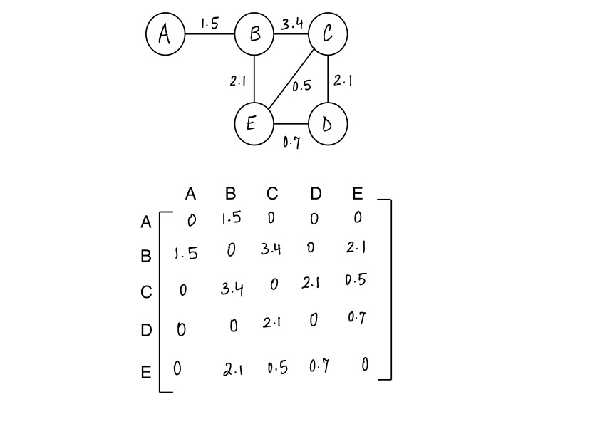

![matrix](images/networks/matrix.png)

Notes: Adjacency list representation and matrix representation. Degree of unwgited vs weighted. Of directed vs undirected graphs.

---

## Matrix representation of graphs

![matrix](images/networks/matrix.png)

What if its an unweighted network?

---
## Matrix representation of graphs

![matrix](images/networks/matrix.png)

What if its a directed network?

---

## Matrix representation of graphs

![matrix](images/networks/matrix.png)

What if it has a self loop?

---
## Matrix representation of graphs

![matrix](images/networks/matrix.png)

What about multiple edges?

---

Note: Another representation is an adjacency list format, though it is less flexible compared to the adjacency matrix representation

---

## Emergent properties of real-world networks

* Presence of hubs: If a network is growing and the property of preferential attachment exists, then the distribution of nodes in the network will assume a "power law" distribution.

* Small world effect: The diameter of the network can be fairly small even in a network with many nodes.

* Robustness: because links are distributed disproportiontately, the failure of any single node will most likely not have a serious impact on the functioning of the network, making real-world networks "robust"

Notes: preferential attachment exists (that is, new nodes are free to associate with any node, but "prefer" to associate with well-connected nodes -- nodes that already have many connections). -- a few nodes have many links, and many nodes have few links. There is no meaningful "average", hence these are sometimes called "scale-free" networks. Remember, because of the importance of superconnectors, real-world networks can be vulnerable to targeted attacks.

---

## Centrality measures in networks

How important is a node/edge to the structural characteristics of the system?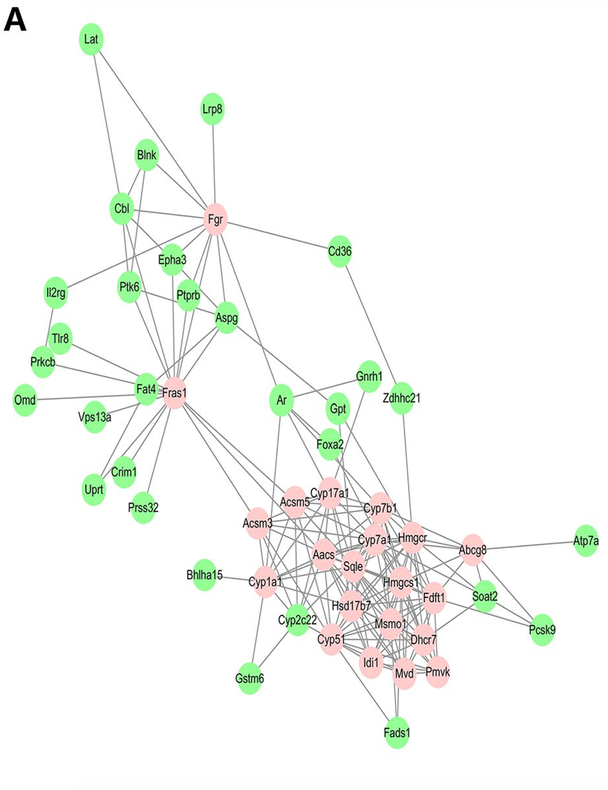

![example](images/networks/centrality_example.png)

<small>Source: PMC6762067</small>

Notes: Several nodes show high conenctivity, but nodes with lower connectivity can still be important. For example, CD36 is a negative regulator of angiogenesis in endothelial cells, though it is not densely connected.

---

## Degree centrality

![degree](images/networks/degree.png)

What about weighted or directed graphs?

---

## Betweenness centrality

The number of shortest paths in the graph that pass through the node divided by the total number of shortest paths.

$BC(k) = \sum_i \sum_j \frac{\rho(i,k,j)}{\rho(i,j)}, i \neq j \neq k$

---

## Betweenness centrality
The number of shortest paths in the graph that pass through the node divided by the total number of shortest paths.

![betweenness](images/networks/betweenness.png)

Shortest paths: AB,ABC,ABCD,ABE,BC,BCD,BE,CD,CE,DE

$BC(B) = 3/10$

Nodes with a high betweenness centrality control information flow in a network.

---

## Closeness centrality

The normalised inverse of the sum of topological distances in the graph.

$CC(i) = \frac{N-1}{\sum_j d(i,j)}$

![betweenness](images/networks/betweenness.png)

$CC(B) = 4 / 5$

Nodes with a high closeness centrality can spread information easily.

Notes: N is the number of nodes

---

## Degree centrality can be different from closeness or betweenness

![example](images/networks/centrality_example.png)

<small>Source: PMC6762067</small>

---

## Eigenvector centrality

Make $x_i$ proportional to the average of the centralities of $i$'s neighbors

$x_i = \frac{1}{\lambda} \sum_{j=1}^{n} A_{ij}x_j$

In matrix-vector notation, we can write $X = \frac{1}{\lambda} AX$ or $AX = {\lambda}X$

Connections to high-scoring nodes contribute more to the score of the node in question than equal connections to low-scoring nodes.

Note: eigenvector v of a linear transformation T is scaled by a constant factor  λ when the linear transformation is applied to it:

---

## Centrality measures in networks

1. Degree centrality: number of in/out edges for $v$
2. Closeness centrality: mean distance to other vertices
3. Betweenness centrality: # of shortest paths
4. Eigenvector centrality: sums of centrality of $v$'s neighbors
5. Katz centrality: balances #1 and #4 using a weighting parameters

6. Page rank: dilutes centrality flow out of a vertex by its number of neighbor

7. ...

8. ...

---

---

## Protein functional distance in networks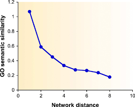

![Distance](images/networks/msb4100129-fig-0003-m.jpg)

<small>Source: PMC1847944</small>

Note: Correlation between protein functional distance and network distance. X‐axis: distance in the network. Y‐axis: average functional similarity of protein pairs that lie at the specified distance. The functional similarity of two proteins is measured using the semantic similarity of their GO categories

---

## Guilt by association

![GBA](images/networks/msb4100129-fig-0002-m.jpg)

<small>Source: PMC1847944</small>

Note: Direct versus module‐assisted approaches for functional annotation. The scheme shows a network in which the functions of some proteins are known (top), where each function is indicated by a different color. Unannotated proteins are in white. In the direct methods (left), these proteins are assigned a color that is unusually prevalent among their neighbors. The direction of the edges indicates the influence of the annotated proteins on the unannotated ones. In the module‐assisted methods (right), modules are first identified based on their density. Then, within each module, unannotated proteins are assigned a function that is unusually prevalent in the module. In both methods, proteins may be assigned with several functions.

---

## Random walks

![Random walk](images/networks/start_0.png)

---

## Random walks

![Random walk](images/networks/start_1.png)

---

## Random walks

![Random walk](images/networks/start.png)

---

## Random walks

![Random walk](images/networks/random_walk.gif)

---

## Random walks

![Random walk](images/networks/random_walk_some_restart.gif)

---

## Random walks

![Random walk](images/networks/random_walk_lots_restart.gif)

---

## Random walks

$A$ : adjacency matrix

$W$ : normalized version of $A$

$p_t = Wp_{t-1}$

With restart probability $c$

$p_t = cp_0 + (1 - c)Wp_{t-1}$

---

## Random walks with restart

![Random walk](images/networks/random_walk_algo.png)

<small>Source: 10.1145/1134030.1134042</small>

---

## Diffusion models

* Model continuous fluid flow over time instead of discrete time steps
* Similarity matrix: $e^{-\alpha W}$ where $W =D - A$

![Diffusion](images/networks/diffusion.png)

<small>Source: 10.1038/nrg.2017.38</small>

---

## Network Propagation

![Propagation](images/networks/network_propagation.png)

<small>Source: 10.1038/nrg.2017.38</small>

Note: Network propagation approaches take a vector the entries of which (0 or 1 or real‐values) indicate the prior information on each gene or node in the network. Following propagation, the scores on the nodes are examined using different approaches. a | 1D approaches rank or prioritize genes by their propagated scores. b | 2D approaches analyse a similarity matrix defined by the propagation and extract modules, or subnetworks, according to both the propagated scores and the topology of the network. c | Integrative approaches propagate prior information from different data sets, or individuals, across one or more networks, forming integrated scores that are used to rank genes and/or to extract modules

---

## Network Propagation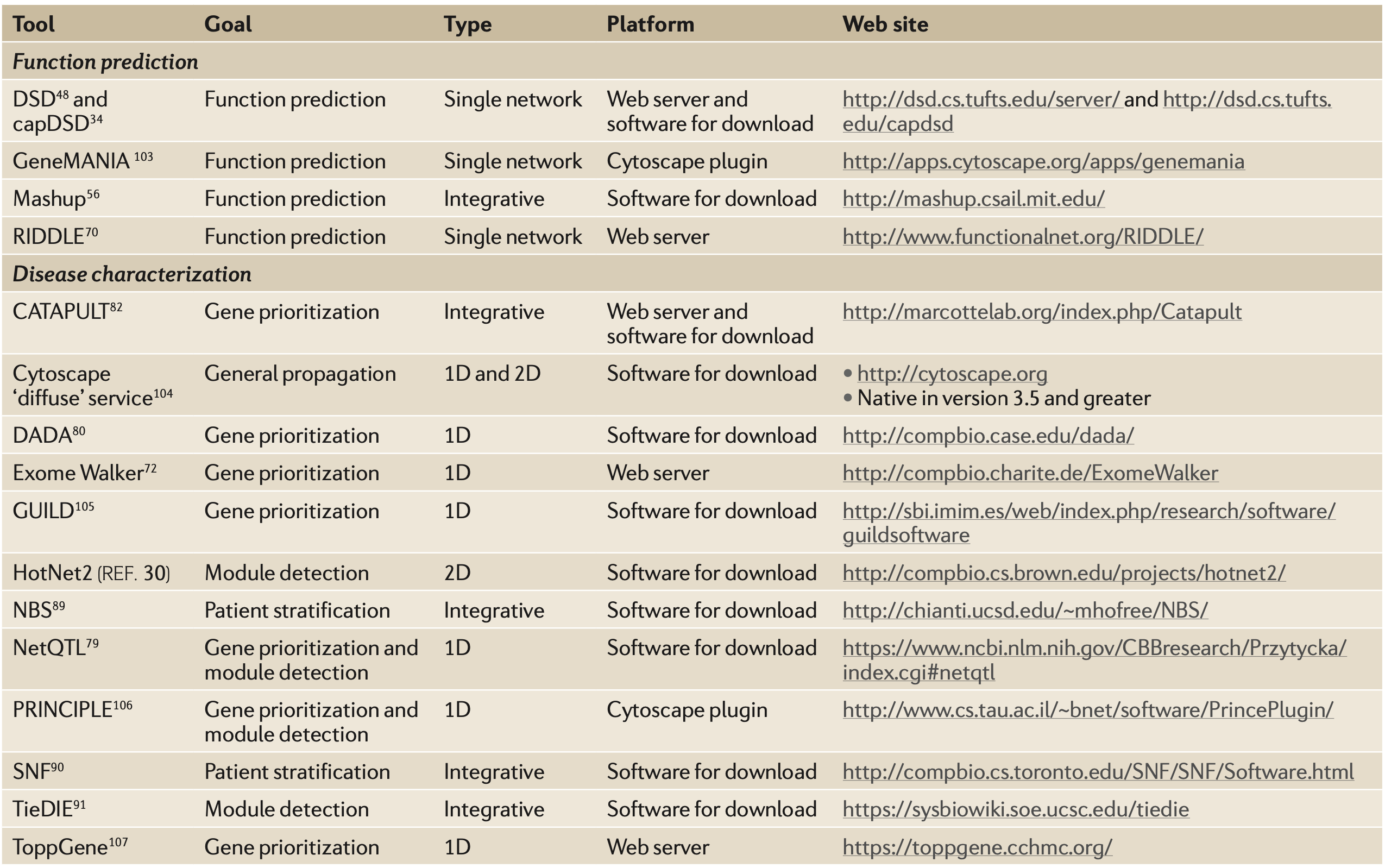

![table](images/networks/propagation.png)

<small>Source: 10.1038/nrg.2017.38</small>

---

---

## Modularity of networks

Modular: Graph with densely connected subgraphs. Genes in modules are involved in similar functions and are co-regulated.

![modular](images/networks/modular.png)

Modules can be identified using graph partitioning algorithms

---
## Community detection

* Node-Centric Community
    * Each node in a group satisfies certain properties
* Group-Centric Community
    * Consider the connections within a group as a whole. The group has to satisfy certain properties without zooming into node-level
* Network-Centric Community
    * Partition the whole network into several disjoint sets
* Hierarchy-Centric Community
    * Construct a hierarchical structure of communities

---

## Node-Centric : Cliques

Clique: a maximum complete subgraph in which all nodes are adjacent to each other

![clique](images/networks/clique.png)

* Most versions of the clique problem are hard
* The clique decision problem is NP-complete (input: G,k output: T/F)
* listing all maximal cliques may require exponential time
* in clique of size $k$, each node mantains degree $\geq k-1$

Notes: NP-complete problems are the hardest of the problems to which solutions can be verified quickly. A maximal clique, sometimes called inclusion-maximal, is a clique that is not included in a larger clique. A single maximal clique can be found by a straightforward greedy algorithm. Starting with an arbitrary clique (for instance, any single vertex or even the empty set), grow the current clique one vertex at a time by looping through the graph's remaining vertices. For each vertex v that this loop examines, add v to the clique if it is adjacent to every vertex that is already in the clique, and discard v otherwise. This algorithm runs in linear time.

---

## Group-Centric Community

Whole group should satisfy a certain condition, e.g., group density $\geq t$

* Subgraph $G_s (V_s, E_s)$ is $\gamma - dense$ quasi-clique if $$\frac{2|E_s|}{|V_s|(|V_s| - 1)} \geq \gamma$$ 
* denominator is the maximum number of degrees
* A strategy similar to that of cliques can be used

---

## Network-Centric Community Detection

consider the connections within a network globally. Partition the nodes of the network into disjoint sets.

* Laplacian matrix $L = D - A$
* For undirected networks
    * diagonal has degree of the node
    * non-diagnoal elements are negative of the adjacency matrix
* graph analogue to the Laplacian operator on multivariate, continuous functions

Notes: the Laplace operator or Laplacian is a differential operator given by the divergence of the gradient of a scalar function on Euclidean space. In a Cartesian coordinate system, the Laplacian is given by the sum of second partial derivatives of the function with respect to each independent variable. In other coordinate systems, such as cylindrical and spherical coordinates, the Laplacian also has a useful form. Informally, the Laplacian Δf (p) of a function f at a point p measures by how much the average value of f over small spheres or balls centered at p deviates from f (p).

---

## Laplacian

Given a multivariate function $f : \mathbb{R}^n \rightarrow \mathbb{R}$, Laplacian of f is defined as

$$\Delta f(x) := \Delta \cdot \Delta f(x)$$

So Laplacian of $f$ is the divergence of f’s gradient.

Note: The gradient of a multivariate function, returns a vector field where the vector at each point x, points in the direction of f’s steepest ascent at x. The divergence operator takes as input a vector field and produces a multivariate function. That is, given a vector field v(x), the divergence at point x, is a scalar that is computed from the vectors that are nearby x in the vector field. Intuitively, the divergence at x describes how much “flow” is coming into and out of x where the flow is described by the vectors in the vector field nearby x. Intuitively, what does the Laplacian describe? Well, following our understanding that f’s gradient provides vectors that point in f’s direction of steepest ascent with magnitude proportional to its steepness, we see that the “flow” at any point in this vector field will correspond to how much the steepness of f is changing. If at some point, x, the steepness is not changing – that is, x is located at a steady incline or a steady decline – then the divergence of the gradient at x will be zero. That is, the Laplacian will be zero. On the other hand, if at x, the steepness is shrinking or growing – for example, because we’re close to a local maximum/minimum – then the divergence (i.e. Laplacian) will be either large or small (large if we’re approaching a minimum and small if we’re approaching a maximum). There exists a whole field dedicated to the study of those matrices, called spectral graph theory

---

## Network modularization

![example](images/networks/modular_example.png)

---

## Network modularization

![example](images/networks/modular_example2.png)

---

## Network modularization

Decompose $L = U \Sigma U^{-1}$

```{R}
L = matrix(c(3,-1,-1, -1, 0,0,0,0,-1,3,-1,-1,0,0,0,0,
            -1,-1,3,-1,0,0,0,0,-1,-1,-1,4,-1,0,0,0,
            0,0,0,-1,4,-1,-1,-1,0,0,0,0,-1,3,-1,-1,
            0,0,0,0,-1,-1,3,-1,0,0,0,0,-1,-1,-1,3), byrow=TRUE, nrow=8)

sorteig <- function(X) {
   vectors <- X$vectors
   values <- X$values
   vectors <- vectors[, order(values)]
   values <- sort(values)
   list(vectors = vectors, values = values)
}

eig <- function(X) {
   res <- eigen(X)
   sorteig(res)
}

eig(L)
```

---

## Network modularization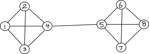

![example](images/networks/modular_example3.png)

```
$vectors
           [,1]       [,2]        [,3]          [,4]          [,5]       [,6]
[1,] -0.3535534  0.3825277  0.83926025  0.000000e+00  0.000000e+00  0.0000000
[2,] -0.3535534  0.3825277 -0.39356606  0.000000e+00 -7.791716e-17 -0.4218144
[3,] -0.3535534  0.3825277 -0.28941826  0.000000e+00 -2.967711e-17 -0.1621762
[4,] -0.3535534  0.2470177 -0.15627594  0.000000e+00  1.075943e-16  0.5839905
[5,] -0.3535534 -0.2470177 -0.15627594  0.000000e+00  1.075943e-16  0.5839905
[6,] -0.3535534 -0.3825277  0.05209198  8.756053e-17  8.164966e-01 -0.1946635
[7,] -0.3535534 -0.3825277  0.05209198 -7.071068e-01 -4.082483e-01 -0.1946635
[8,] -0.3535534 -0.3825277  0.05209198  7.071068e-01 -4.082483e-01 -0.1946635
            [,7]       [,8]
[1,] -0.06305206 -0.1426158
[2,] -0.61279013 -0.1426158
[3,]  0.77347870 -0.1426158
[4,] -0.09763651  0.6625573
[5,] -0.09763651 -0.6625573
[6,]  0.03254550  0.1426158
[7,]  0.03254550  0.1426158
[8,]  0.03254550  0.1426158

$values
[1] -6.383782e-17  3.542487e-01  4.000000e+00  4.000000e+00  4.000000e+00
[6]  4.000000e+00  4.000000e+00  5.645751e+00
```

Note: number of times 0 appears as an eigenvalue in the Laplacian is the number of connected components in the graph. Second eigenvalue called the algebraic connectivity, is greater than 0 if and only if G is a connected graph, and reflects how well connected the overall graph is. Second eigenvector of Laplacian matrix characterizes a network partition. So all positive values in this case are one cluster, and the negative values are the second cluster

---

---

## Outline

* Introduction to networks
    * Representations
* Global/Local network properties
    * Emergent properties
    * Centrality
* Guilt by association
    * Direct methods
    * Module-assisted

---