reveal.js

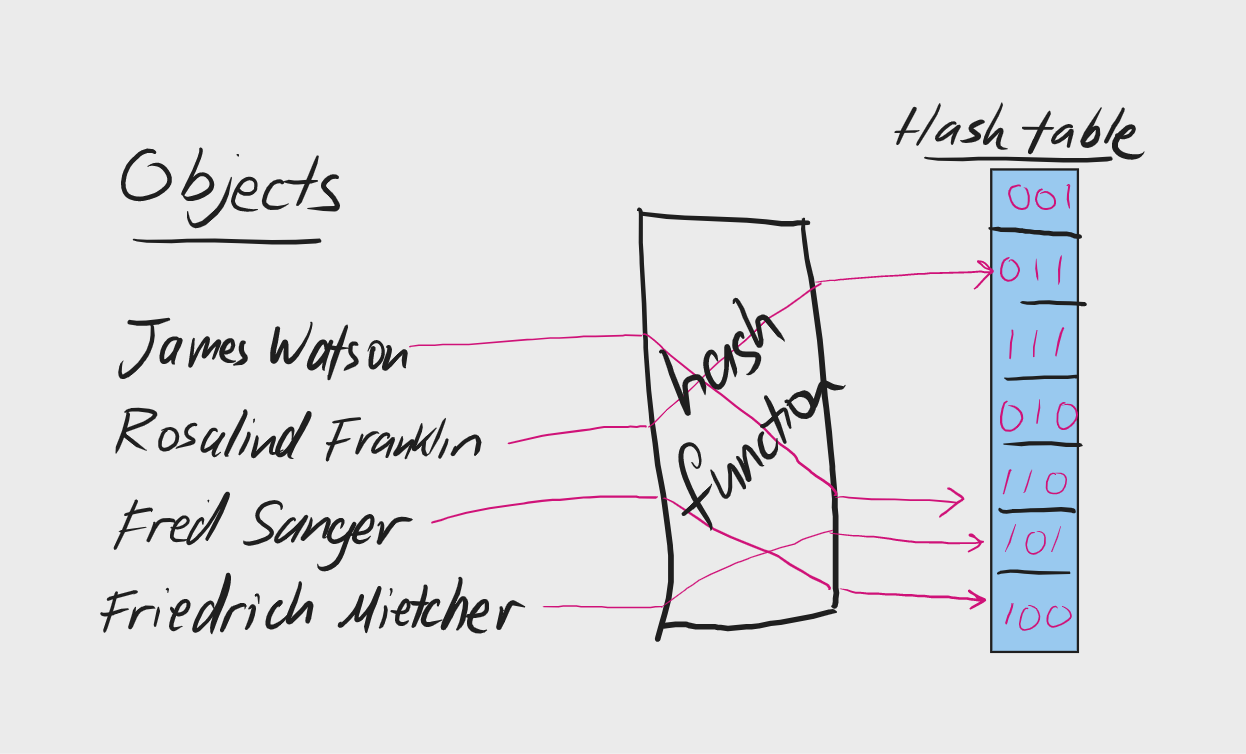
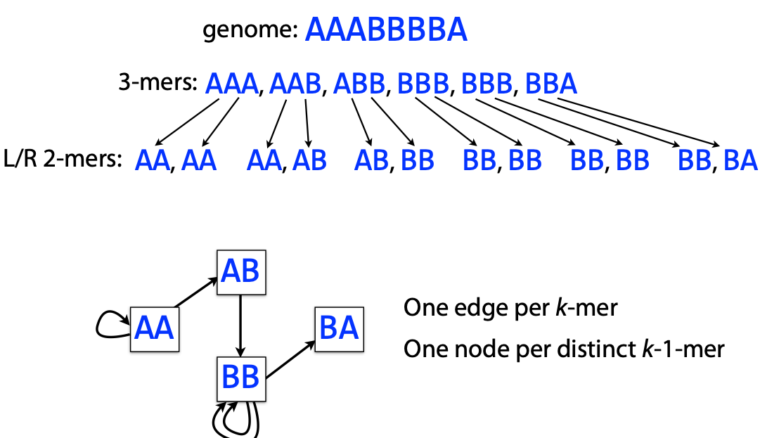
## RNA-seq pseudoalignment, K-mers, and Hashing
---
## Lecture overview

- RNA quantification with EM
- RNA pseudoalignment
- K-mer counting
- Hashing and MinHash
- Bloom filters

---
### Intro to RNA-seq

---
### Transcript models
<img src="images/genomic-intervals/brca2-gene-model.png" height="320">

RNA analysis may include:
- de novo assembly
- pre-existing fixed set for quantification

---
### Review of EM

- Expectation Maximization is an algorithm to find Maximum Likelihood Estimates
- It is used in situations where there is missing data
- Missing data may be either intentional or unintentional
- Intentional missing data is used for mixture models

---
### EM for mixture models

$$
P(\mathbf{X}) = \prod_{i=1}^{N} \sum_{k=1}^{K} \pi_k  P(X_i=x | \theta_k)
$$

$P(\mathbf{X})$ is the joint probability of observed data $\mathbf{X}$  
$\pi_k$ are the mixture parameters  
$\theta_k$ are the model parameters for each component

Latent indicator/responsibility variable $Z_{ik}$ is introduced to assign data $i$ to component $k$.

</div>

---
### EM in RNA-seq

- Observed data is a set of aligned reads $R$
- Latent mixture vars $Z$ assigns $R_j$ to transcript $T_i$
- We want to infer expression of each transcript $\theta_i$
- See: [Li 2010](https://doi.org/10.1093/bioinformatics/btp692) and [Li 2011](https://doi.org/10.1186/1471-2105-12-323)

#### Expectation (E-step)

Guess assigning reads to transcripts ($E[Z]$)

#### M-step

Calculate expression values ($\Theta$) for each transcript

---
### Expectation (E-step)

Guess assigning reads to transcripts ($E[Z]$)

#### E-step detail

$E[Z] = P(Z=1|r,\theta_{i}^{old})$

- $Z_{ij}$ is the probability that read $j$ was drawn from transcript isoform $i$.
- $Z$ is huge ($|R| \times |T|$), but we can use alignment to constrain it (fix some at $0$).

---

#### E-step detail

Just assign the read to the transcript according to its abundance estimate $\theta_i$

$E[Z] = P(Z=1|r,\theta_{i}^{old})$

$E[Z_{ij}] = \frac{\theta_i^{old}}{\sum_{i|Z_{ij}\not=0}{\theta_i^{old}}}$

- Uniquely aligning reads are assigned to 1 isoform, $E[Z_{ij}]=1$
- Multi-aligning reads are assigned proportionally to the expression estimates $\Theta$, for compatible transcripts.

---
### M-step

Calculate expression values ($\Theta$) for each transcript

$\argmax_{\Theta} \cal L(\theta_{i} | Z, r)$

#### M-step detail

- We want to infer $\Theta = [\theta_1, \theta_2, ..., \theta_n]$
- $\theta_i$ measures expression for isoform $i$

$\theta_i^{new} = \frac{\sum_j^R{Z_{ij}}}{N}$

---
### Summary of EM for RNA-seq

E-step: Assigning reads to transcripts ($E[Z]$)

$E[Z] = \frac{\theta_i^{old}}{\sum_{i}{\theta_i^{old}}}$

M-step: Calculate expression ($\Theta$) for each transcript

$\theta_i^{new} = \frac{\sum_j^R{Z_{ij}}}{N}$

<div class="fragment">
  Traditionally uses read-transcript alignments
</div>

---
# K-mers

---
### k-mers: subsequences of length *k*

![](images/k-mer-analysis/3-mers.svg)

</div>
<div class="col">
<h2>2-mers</h2>

![](images/k-mer-analysis/2-mers.svg)

</div>
</div>
---
How many 7-mers are there  
in a sequence with $l=11$ bases?

<div class="fragment">
$x = l-k+1 = 5$

```
|ABCDEFGHIJK|
|1-----7    | 1
| 1-----7   | 2
|  1-----7  | 3
|   1-----7 | 4
|    1-----7| 5
```
</div>

<div class="fragment">
  This is total k-mers, not unique k-mers
</div>

---
### Exponential growth

$4^k$

```
> cbind(k=seq(1,20), combinations=4^seq(1, 20))
       k  combinations
 [1,]  1             4
 [2,]  2            16
 [3,]  3            64
 [4,]  4           256
 [5,]  5          1024
 [6,]  6          4096
 [7,]  7         16384
 [8,]  8         65536
 [9,]  9        262144
[10,] 10       1048576
[11,] 11       4194304
[12,] 12      16777216
[13,] 13      67108864
[14,] 14     268435456
[15,] 15    1073741824
[16,] 16    4294967296
[17,] 17   17179869184
[18,] 18   68719476736
[19,] 19  274877906944
[20,] 20 1099511627776
```

---
Human chromosome 1 has 248,956,422 bp.

> Assuming a random distribution of 4 bases, what is the expected count of a given 7-mer on human chromosome 1?

---

$l = 248,956,422$ size of chr1  
$l-k+1 = 248,956,416$ total 7-mers in chr1

$4^7 = 16384$ possible 7-mer types  
$ 248,956,416 / 16384 \approx \mathbf{15195} $

---
## Kmers and motifs
<div class="row">
<div class="col">
<h2>K-mer</h2>

![](images/k-mer-analysis/3-mers.svg)

</div>
<div class="col">
<h2>Motif</h2>

- A k-mer is like a simplified motif with no weights
- K-mers are faster to compute and require less data
- K-mers represent a single instance, rather than a set
---
## Applications of K-mers
- Alignment seeds (fast RNA counting)
- Counting for relationships (e.g. metagenomics)
- Dinucleotide/codon analysis, background models
- Sequence assembly (De Bruijn graphs)
- Simplified transcription factor binding
- RNA pseudoalignment

---
## K-mer Counting

![](images/k-mer-analysis/k-mer-counting.svg)

<div class="mermaid" style="display:none">
graph TD
  GATTACAGATTCAG-->GAT;
  GATTACAGATTCAG-->ATT;
  GATTACAGATTCAG-->TTA;
  GATTACAGATTCAG-->TAC;
  GATTACAGATTCAG-->ACA;
  GATTACAGATTCAG-->ATT;
  GATTACAGATTCAG-->CAG;
  GATTACAGATTCAG-->AGA;
  GATTACAGATTCAG-->TTC;
  GATTACAGATTCAG-->TCA;
  GATTACAGATTCAG-->CAG;
  GAT-->n([1]);
  ATT-->n2([2]);
  TTA-->n3([1]);
  TAC-->n4([1]);
  ACA-->n5([1]);
  CAG-->n6([2]);
  AGA-->n7([1]);
  TTC-->n8([1]);
  TCA-->n9([1]);
</div>

K-mer counting converts a sequence into a vector

![](images/k-mer-analysis/k-mer-vector.svg)

<div class="mermaid" style="display:none">
graph LR
  GATTACAGATTCAG-->n1["1 2 1 1 1 1 2 1 1 1"];
  CTGAGGACTCGACT-->n2["2 1 0 0 2 2 3 2 2 1"];;
</div>

---

Remember: $4^k$

```
> cbind(k=seq(1,20), combinations=4^seq(1, 20))
       k  combinations
 [8,]  8         65536
 [9,]  9        262144
[10,] 10       1048576
[11,] 11       4194304
[12,] 12      16777216
[13,] 13      67108864
[14,] 14     268435456
[15,] 15    1073741824
[16,] 16    4294967296
[17,] 17   17179869184
[18,] 18   68719476736
[19,] 19  274877906944
[20,] 20 1099511627776
```

High $k$ $\rightarrow$ high-dimensional vectors, sparsity

---

### Hashing

> A hash function maps an object to a finite space

- must be deterministic
- should be very fast to compute
- should reduce collisions

Uses of hash functions

1. Hash table keys
2. Evaluating similarity (or identity)
3. Cryptography

---
![](images/k-mer-analysis/hash_function.png)

---

### Hash tables
- provide $O(1)$ complexity for item access
- Can store large objects for lookup with a key

---
### Cryptographic hash function
- a subset of hash functions with particular purposes:
  - designed to go one way (hard to de-hash)
  - designed to avoid collisions
  - relies on the avalanche effect (small change in inputs leads to large change in output)

---
### md5 algorithm- "Message Digest"

In 2011, the Internet Engineering Task Force (IETF) [advised in this document](https://tools.ietf.org/search/rfc6151) that

> The published attacks against MD5 show that it is not prudent to use MD5 when collision resistance is required.

---
## MinHash

MinHash uses hashing to determine similarity between two sets very quickly.

Jaccard index measures similarity between two sets

$$
J(A,B) = \frac{|A \cap B|}{|A \cup B|}
$$

Computing can be time-consuming for large sets

</div>

MinHash estimates the Jaccard index rapidly, using hashing to avoid computing intersection and union

</div>

---
### MinHash

$U$ is the universe of elements

Hash function $h$ maps set elements to unique integers

$h(x): U \rightarrow \mathbb{Z}$

Given a subset $S \subset U$, $h_{min}(S)$ is the minimum hash value (integer) $h(e_i)$ for each element $e_i \in S$.

---

$h_{min}(A) = h_{min}(B)$

if and only if the element with minimum hash value in $U = A \cup B$ is also in $A \cap B$.

The probability of this is $J(A,B) = \frac{|A \cap B|}{|A \cup B|}$.  
So $P(h_{min}(A) = h_{min}(B))$ is an estimator of $J$.

</div>

But we need more than one draw:
- multiple hash functions
- take the $n$ lowest as the MinHash *signature* or *sketch*

</div>

---

MinHash has been used for fast comparisons of DNA sequences with k-mers.

- Metagenomics ([Ondov 2016](https://doi.org/10.1186/s13059-016-0997-x))
- Sourmash ([Brown 2016](https://doi.org/10.21105/joss.00027))
- Phylogenetics ([Moi 2020](https://doi.org/10.1371/journal.pcbi.1007553))
- Genome assembly ([Berlin 2015](https://doi.org/10.1038/nbt.3238) and [Koren 2017](https://doi.org/10.1101/gr.215087.116 ))

---

## Bloom filters

- Probabilistic membership testers using hash tables
- Fast and memory efficient

- Guarantee an item *is not* in the set, but not if it is (false positives allowed)
- Elements cannot be removed from the set

---
### Bloom filter components

1. A bit vector $F$ of length $l$ (size of the filter)
2. $k$ hash functions $h_i(x): U \rightarrow \mathbb{Z}$, $i \in 1, 2, ..., k$, which map objects in the universe $U$ to integers $\mathbb{Z}$ in $(0, l]$.

Parameters:

- Size $l$: how many elements in the bit vector?
- Number of hash functions
- Hash functions themselves

---
### Bloom filter procedure: add

A Bloom filter represents a set of elements $S \subset U$

To add an element $e$:

1. Compute the $k$ hash functions, $h_i(e), ...$
2. Set $F[h_i(e)] = 1$ for $i \in 1:k$.

---
### Bloom filter procedure: test

To test for presence of an element $e$:

1. Compute the $k$ hash functions, $h_i(e), ...$
2. Test $F[h_i(e)] \overset{?}{=} 1$ for $i \in 1:k$.

3. if $\forall i \in [1, k]: F_i=1$, then $e \overset{?}{\in} S$.  
Otherwise, $e \not\in S$.

---
![](images/k-mer-analysis/bloom_filters.svg)

---
## A basic hash function

$h(x): U \rightarrow \mathbb{Z}$, $\mathbb{Z} \in (0, l]$

```R
hashfunc = function(d) {
  hash = 0
  r = as.integer(charToRaw(d))  # convert char to int
  for (item in r) {
    hash = hash * 7 + item
  }
  hash %% 1024
}

```

---
## Hash function considerations

- uniformity of hash values
- more functions affects speed, accuracy, and fill rate

[Kirsch-Mitzenmacher optimization](https://www.eecs.harvard.edu/%7Emichaelm/postscripts/tr-02-05.pdf)

Given 2 hash functions $h_1(x)$ and $h_2(x)$, simulate additional values with $g_i(x) = h_1(x) + i * h_2(x)$, $i \in [0, k-1]$ for $k$ additional hash functions.

</div>

---

### Bloom filters in practice

- RNA-seq quantification ([Zhang 2014](https://doi.org/10.1093/bioinformatics/btu288))
- Pre-alignment species filtering ([Chu 2014](https://doi.org/10.1093/bioinformatics/btu558))
- Single-cell transcriptome assembly ([Nip 2020](https://doi.org/10.1093/10.1101/gr.260174.119))
- Large-scale transcript searching ([Solomon 2016](https://doi.org/10.1038/nbt.3442))
- Genome assembly ([Jackman 2017](10.1101/gr.214346.116 ))
- Review of [Sketching and Sublinear Data Structures in Genomics](https://www.annualreviews.org/doi/abs/10.1146/annurev-biodatasci-072018-021156)

---
## RNA Pseudoalignment

Quantifying expression...

- only requires an assignment of reads to transcripts
- therefore doesn't require a complete alignment
- could be sped up by assigning reads without computing an alignment

---
## RNA Pseudoalignment

Build index: 
1. de Bruijn graph
2. contigs
3. k-mer index

Pseudo-align reads:
1. Contig lookup
2. Intersection

---
Transcriptome de Bruijn graph (T-DBG)

![](images/genome_assembly/debruijn.png)

---
### Kallisto

- each node corresponds to a k-mer (default k=31)
- isoforms are overlaid on the graph

---

<a href="https://www.nature.com/articles/nbt.3519/figures/1"><img src="images/k-mer-analysis/kallisto_fig1c.png" width="400"></a>
- linear stretches with the same isoforms are 'contigs'
- Build Index: A hash table maps the K-mer to contigs

Align:
1. Look up compatibility class for each k-mer in read
2. Intersect them.

</div>

---

### Quantify

$$
\cal L(\alpha) \propto \prod_{r \in R} \sum_{t \in T} y_{rt} \frac{\alpha_t}{l_t}
$$

reads $r \in R$,  
transcripts $t \in T$,  
compatibility matrix $y_{rt}$,  
expression levels $\alpha_t$ for transcript $t$ with length $l$

---
## Pseudoalignment summary

Assign reads to transcript with fast k-mer hash tables.

Use EM to iteratively compute assignments $Z$ (E-step)

Then maximize by computing expression levels $\Theta$