Remember this?

Lower costs → More data

Scalable computing in genomics

Genomics can be 'big data'.

Component of scalability: 1) time and 2) space

Typical epigenome project

Many independent samples (patients, cell lines, conditions)
2 Analysis stages:
1. "Pipeline": Processing raw data
2. "Analysis": Analyzing processed data

Approaches for scalability

Parallelization
Optimization
Compression
Databases

1. Parallelization

Splitting a compute task, and then completing each split simultaneously.

split-apply-combine

Many problems call for a similar computing architecture
e.g. MapReduce/Hadoop

Scopes of parallelism

by process

by sample

by dependence

Parallel by process

PROs:

easy to use if the tool can do it (e.g. -c 16)
relatively easy in R or Python

CON:

node-threaded parallelism (restricted to a single node)
typically built-in to a tool, so limited by tool capacity

Aside: Cluster hardware

Parallel by sample/job

PRO:

no shared memory; limited only by cluster size
HPC clusters are intended for this type of parallelization
Restricted by size of HPC, rather than node (burst to cloud)
Doesn't depend on the tool

CON:

requires independence of jobs

Parallel by dependency

PRO:

not necessarily node-threaded

CON:

may have shared file-system requirements
requires a dependency graph of workflow steps
requires a layer of task management above typical HPC usage
limited to independent workflow elements
requires independence of jobs

Scopes of parallelism: tradeoffs

by process

by sample

by dependence

Very easy

Easy

Hard

Parallel jobs in R

BatchJobs
snow

Parallel processing in R

parallel package (part of Core R)

lapply(data, func)  # serial
mclapply(data, func, mc.cores=detectCores())  # parallel

Parallel processing in Python

subprocess module

import subprocess

>>> subprocess.run(["ls", "-l"])  # doesn't capture output
CompletedProcess(args=['ls', '-l'], returncode=0)

>>> subprocess.run(["ls", "-l", "/dev/null"], capture_output=True)
CompletedProcess(args=['ls', '-l', '/dev/null'], returncode=0,
stdout=b'crw-rw-rw- 1 root root 1, 3 Jan 23 16:23 /dev/null\n', stderr=b'')

multiprocessing module

from multiprocessing import Pool

def f(x):
    return x*x

if __name__ == '__main__':
    with Pool(5) as p:
        print(p.map(f, [1, 2, 3]))

Workflows

A workflow or pipeline is a repeatable sequence of tasks that process a piece of data.

Workflow spectrum

Workflow/pipeline engine/framework

A development toolkit that makes it easier to build workflows.

Snakemake
Nextflow
Common Workflow Language

Snakemake

SAMPLES = ["A", "B"]


rule all:
    input:
        "plots/quals.svg"


rule bwa_map:
    input:
        "data/genome.fa",
        "data/samples/{sample}.fastq"
    output:
        "mapped_reads/{sample}.bam"
    shell:
        "bwa mem {input} | samtools view -Sb - > {output}"


rule samtools_sort:
    input:
        "mapped_reads/{sample}.bam"
    output:
        "sorted_reads/{sample}.bam"
    shell:
        "samtools sort -T sorted_reads/{wildcards.sample} "
        "-O bam {input} > {output}"


rule samtools_index:
    input:
        "sorted_reads/{sample}.bam"
    output:
        "sorted_reads/{sample}.bam.bai"
    shell:
        "samtools index {input}"


rule bcftools_call:
    input:
        fa="data/genome.fa",
        bam=expand("sorted_reads/{sample}.bam", sample=SAMPLES),
        bai=expand("sorted_reads/{sample}.bam.bai", sample=SAMPLES)
    output:
        "calls/all.vcf"
    shell:
        "samtools mpileup -g -f {input.fa} {input.bam} | "
        "bcftools call -mv - > {output}"


rule plot_quals:
    input:
        "calls/all.vcf"
    output:
        "plots/quals.svg"
    script:
        "scripts/plot-quals.py"

Nextflow

// Script parameters
params.query = "/some/data/sample.fa"
params.db = "/some/path/pdb"

db = file(params.db)
query_ch = Channel.fromPath(params.query)

process blastSearch {
    input:
    file query from query_ch

    output:
    file "top_hits.txt" into top_hits_ch

    """
    blastp -db $db -query $query -outfmt 6 > blast_result
    cat blast_result | head -n 10 | cut -f 2 > top_hits.txt
    """
}

process extractTopHits {
    input:
    file top_hits from top_hits_ch

    output:
    file "sequences.txt" into sequences_ch

    """
    blastdbcmd -db $db -entry_batch $top_hits > sequences.txt
    """
}

Common workflow language

#!/usr/bin/env cwl-runner

cwlVersion: v1.0
class: Workflow
inputs:
  tarball: File
  name_of_file_to_extract: string

outputs:
  compiled_class:
    type: File
    outputSource: compile/classfile

steps:
  untar:
    run: tar-param.cwl
    in:
      tarfile: tarball
      extractfile: name_of_file_to_extract
    out: [extracted_file]

  compile:
    run: arguments.cwl
    in:
      src: untar/extracted_file
    out: [classfile]

Stop writing shell scripts!

Shell scripting language is difficult to write
As a corollary, shell scripts are also generally difficult to read
Shell scripting lacks the features in a full-service language

The shell makes common and simple actions really simple, at the expense of making more complex things much more complex.

Typically, a small shell script will be shorter and simpler than the corresponding python program, but the python program will tend to gracefully accept modifications, whereas the shell script will tend to get less and less maintainable as code is added.

This has the consequence that for optimal day-to-day productivity you need shell-scripting, but you should use it mostly for throwaway scripts, and use python everywhere else. -Anonymous

Advantages of workflow frameworks

Reproducibility
Restartability
Reusability
Logging
Provenance
Scaling up compute resources
Dependency management

2. Optimization

Algorithm complexity
Language choice and quirks
Time/memory tradeoff

Optimization: algorithm complexity

Source: https://www.bigocheatsheet.com/

How big of data can you handle?

data.frame(C=1, logN=log(n), N=n, NLogN=n*log(n), NSq=n^2, TwotoN=2^n, NFactorial=factorial(n))

   C      logN  N     NLogN NSq  TwotoN          NFactorial
2  1 0.6931472  2  1.386294   4       4                   2
3  1 1.0986123  3  3.295837   9       8                   6
4  1 1.3862944  4  5.545177  16      16                  24
5  1 1.6094379  5  8.047190  25      32                 120
6  1 1.7917595  6 10.750557  36      64                 720
7  1 1.9459101  7 13.621371  49     128                5040
8  1 2.0794415  8 16.635532  64     256               40320
9  1 2.1972246  9 19.775021  81     512              362880
10 1 2.3025851 10 23.025851 100    1024             3628800
11 1 2.3978953 11 26.376848 121    2048            39916800
12 1 2.4849066 12 29.818880 144    4096           479001600
13 1 2.5649494 13 33.344342 169    8192          6227020800
14 1 2.6390573 14 36.946803 196   16384         87178291200
15 1 2.7080502 15 40.620753 225   32768       1307674368000
16 1 2.7725887 16 44.361420 256   65536      20922789888000
17 1 2.8332133 17 48.164627 289  131072     355687428096000
18 1 2.8903718 18 52.026692 324  262144    6402373705728000
19 1 2.9444390 19 55.944341 361  524288  121645100408832000
20 1 2.9957323 20 59.914645 400 1048576 2432902008176640000

Factorial time $O(n!)$

Factorial time arises in problems involving permutations

Traveling salesman: find the minimum distance path connecting all points.

Source: Travelling salesman problem

Factorial time $O(n!)$

Shortest common superstring: Given set of strings S find shortest string containing the strings in S as substrings

Brute force: enumerate all orders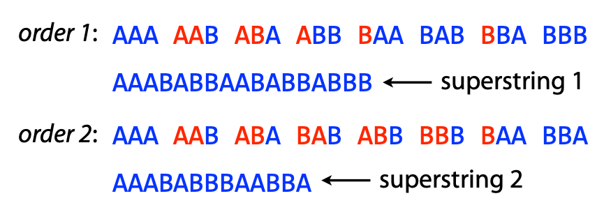

Which is worse?

$O(c^n)$ - Exponential time
$O(n^c)$ - Polynomial time

Exponential time $O(2^n)$

Exponential time arises in problems with nested subproblems

Longest common subsequence (LCS): find the longest subsequence common to all sequences in two sequences.

def longest_cmn_subseq(s1, s2, ind1, ind2):
    if (ind1 == -1 or ind2 == -1):  # base case
        return 0
    if (s1[ind1] == s2[ind2]):  # match
        return 1 + longest_cmn_subseq(s1, s2, ind1-1, ind2-1)
    return max(longest_cmn_subseq(s1, s2, ind1-1, ind2), longest_cmn_subseq(s1, s2, ind1, ind2-1))

longest_cmn_subseq("TCGA", "TGCTA", 3, 4)
3

Exponential time comes from the double recursive call

Polynomial time $O(n^2)$

Nested loops

# Naively align reads to a reference genome
for (r in reads):  # Order 10^8 ?
    for (p in reference_positions): # Order 10^9
        score_alignment(r, p)

# Scan for motif matches
for (m in motifs): # Order 10^3
    for (s in sequences): # Order 10^7
        motif_scan(m, s)

Find the overlaps

Sequential search: $O(n)$ - Linear time
Binary search $O(log(n))$ - Logarithmic time

Constant time $O(1)$

Array lookup

regions[15]

Indexes

regions[ index(chr1, 1526) ]

Tabix indexing

Input:

chr1    10468   annotation1
chr1    10469   annotation2
chr1    10470   annotation3

Compress: bgzip file.tsv
Index: tabix -s 1 -b 2 -e 2 file.tsv.gz
Retrieve: tabix file.tsv.gz.tbi chr5:50000-100000

See Tabix Bioinformatics paper

Optimization: Language choice

Existing implementations are often faster than yours
Compiled languages are faster than scripting languages
Loops in R are slow

Use vectorized loops in R

library("microbenchmark")
d = matrix(rnorm(10000000), 10, 1000000)
myMeans = function(d) {
    means = c()
    for (i in 1:ncol(d)) {        means[i] = mean(d[,i])    }
    means
}

microbenchmark(    
    myMeans(d),
    apply(d, 2, mean),
    colMeans(d),
    times=3)

Unit: milliseconds
              expr  min   lq mean median   uq   max neval
        myMeans(d) 4693 4880 4997   5067 5149  5230     3
 apply(d, 2, mean) 4856 5047 5152   5237 5300  5363     3
       colMeans(d)    7    7    7      7    7     8     3

Link C code into R or Python

Rcpp makes it easy to link C++ into R.
Extending Python shows how to call C extensions from Python
Cython compiles Python code into C extensions

Optimization: Speed/memory tradeoff

Disk I/O is a often bottleneck.
Prevent reads/writes by loading into memory.
Memory lookups are quick

Extract ATAC in consensus peaks

Method 1 pseudocode:

def quantify_accessibility(peaks_bed, reads_bam):
    with(f as open(peaks_bed)):
        count_reads(f.readline(), readsbam)

Method 2 pseudocode:

def quantify_accessibility(peaks_bed, reads_bam):
    peaks = load_file(peaks_bed)
    for (r in peaks):
        count_reads(r, readsbam)

Which is faster? Which uses more memory?

Could we switch the peaks and reads?

Aside: Cluster hardware

Compression

Does smaller = faster ?

Zipping files leads to faster transfer
But zipping files must be unzipped to be read
But loading less data off disk is faster
Disk space vs compute time is also a tradeoff

GZIP

Based on LZ77 and Huffman Coding

Run-length Encoding

> c(rep(1,20), rep(0,15))
 [1] 1 1 1 1 1 1 1 1 1 1 1 1 1 1 1 1 1 1 1 1 0 0 0 0 0 0 0 0 0 0 0 0 0 0 0
> rle(c(rep(1,20), rep(0,15)))
Run Length Encoding
  lengths: int [1:2] 20 15
  values : num [1:2] 1 0

LZ77

Duplicate string elimination

Find the longest repeated sequences in string
Replace repeats with relative references to earlier

Input: "The compression and the decompression leave an impression. Hahahahaha!"

Output: "The compression and t [20 | 3] de [22 | 12] leave [28 | 3] i [42 | 7] . Hah [2 | 7] !"

Example credit: https://sudonull.com

Huffman Coding

Minimum redundancy codes: assign the fewest bits to the most common characters.

DNA Input: ACTGAACGATCAGTACAGAAG

Base   Freq     ASCII   2bit  HuffCode    
   A      9  01000001     00         0    
   G      5  01000111     01        10    
   C      4  01000011     10       110    
   T      3  01010100     11       111

Requires prefix property for variable-width codes
Requires sequential reading (no random access)

See Okaily et al

BAM file format

FASTQ -> SAM
SAM specification. Columns

Example SAM file

@HD VN:1.6 SO:coordinate
@SQ SN:ref LN:45
r001 99 ref 7 30 8M2I4M1D3M = 37 39 TTAGATAAAGGATACTG *
r002 0 ref 9 30 3S6M1P1I4M * 0 0 AAAAGATAAGGATA *
r003 0 ref 9 30 5S6M * 0 0 GCCTAAGCTAA * SA:Z:ref,29,-,6H5M,17,0;
r004 0 ref 16 30 6M14N5M * 0 0 ATAGCTTCAGC *
r003 2064 ref 29 17 6H5M * 0 0 TAGGC * SA:Z:ref,9,+,5S6M,30,1;
r001 147 ref 37 30 9M = 7 -39 CAGCGGCAT * NM:i:1

@HD VN:1.6 SO:coordinate
@SQ SN:ref LN:45
r001 99 ref 7 30 8M2I4M1D3M = 37 39 TTAGATAAAGGATACTG *
r002 0 ref 9 30 3S6M1P1I4M * 0 0 AAAAGATAAGGATA *
r003 0 ref 9 30 5S6M * 0 0 GCCTAAGCTAA * SA:Z:ref,29,-,6H5M,17,0;
r004 0 ref 16 30 6M14N5M * 0 0 ATAGCTTCAGC *
r003 2064 ref 29 17 6H5M * 0 0 TAGGC * SA:Z:ref,9,+,5S6M,30,1;
r001 147 ref 37 30 9M = 7 -39 CAGCGGCAT * NM:i:1

99 = 01100011
 1 = 00000001
 2 = 00000010
32 = 00100000
64 = 01000000

>>> 99 & 0x1
1
>>> 99 & 0x2
2
>>> 99 & 0x4
0
>>> 99 & 0x8
0
>>> 99 & 0x10  # hexadecimal 16
0
>>> 99 & 0x20  # hexadecimal 32
32
>>> 99 & 0x40  # hexadecimal 64
64
>>> 99 & 0x80  # hexadecimal 128
0

Explain SAM flags

@HD VN:1.6 SO:coordinate
@SQ SN:ref LN:45
r001 99 ref 7 30 8M2I4M1D3M = 37 39 TTAGATAAAGGATACTG *
r002 0 ref 9 30 3S6M1P1I4M * 0 0 AAAAGATAAGGATA *
r003 0 ref 9 30 5S6M * 0 0 GCCTAAGCTAA * SA:Z:ref,29,-,6H5M,17,0;
r004 0 ref 16 30 6M14N5M * 0 0 ATAGCTTCAGC *
r003 2064 ref 29 17 6H5M * 0 0 TAGGC * SA:Z:ref,9,+,5S6M,30,1;
r001 147 ref 37 30 9M = 7 -39 CAGCGGCAT * NM:i:1

BAM

BGZF is block compression implemented on top of the standard gzip file format. The goal of BGZF is to provide good compression while allowing efficient random access to the BAM file for indexed queries. The BGZF format is ‘gunzip compatible’, in the sense that a compliant gunzip utility can decompress a BGZF compressed file.

BAM

.bam file contains the aligned read data
.bai file contains the index (offsets to locations of bins)

Aside: BigBed and BigWig

Compressed and Indexed versions of BED and WIG files.
Compressed: makes the files much smaller.
Indexed: Random access allows reading specific chunks

CRAM

"Reference-based" compression (Fritz 2011)
CRAM 3.1 introduced by Bonfield 2022

CRAM 3.1: Bonfield 2022

Although reference compression is where the original work focussed, it is wrong to assume that this is the primary reason for CRAM’s reduced file size. BAM serializes all data together (first name, chromosome, position, sequence, quality and auxiliary fields, then second name, chromosome and so on). This leads to poor compression ratios as names, sequences and quality values all have very different characteristics. CRAM has a column-oriented approach, where a block of names are compressed together or a block of qualities together.

Databases

Database:Space as Parallelization:Compute
They offload storage requirements
They are critical for simultaneous multi-user
Reduce storage requirements by centralizing
Data has gravity, it brings compute to it

Explosion of biomedical cloud platforms

AnVIL [Schatz 2021]
Gabriella Miller Kids First Data Resource Center [Heath 2019]
Cavatica [Volchenboum 2017]
Gen3 Workspaces [Hughes 2019]
Biomedical Research Hub [Barnes 2021]
AHA Precision Medicine Platform [KassHout 2018]
CanDIG [Dursi 2021]
NHLBI BioData Catalyst
Alex's Lemonade Stand Refine.bio
Pediatric Cancer Data Commons [Plana 2021]
SAGE Bionetworks’ Synapse [Grayson 2019]
NCI Genomic Data Commons [Heath 2021]

Problems with cloud platforms

Platform lock-in
Difficulty integrating across platforms
Duplicated effort for both users and developers