## Bayes theorem, Likelihood, and Expectation-Maximization 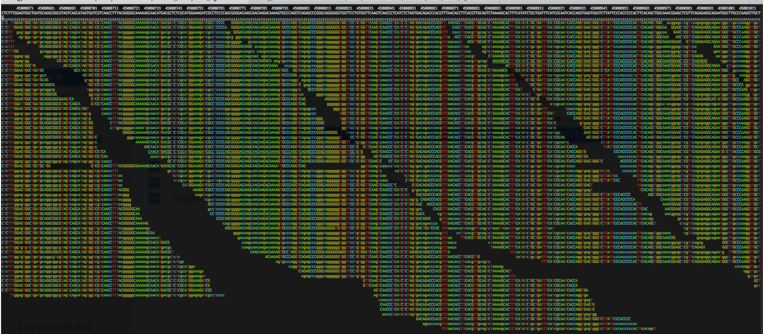 --- ## Alignments expose differences  --- ## Types of differences 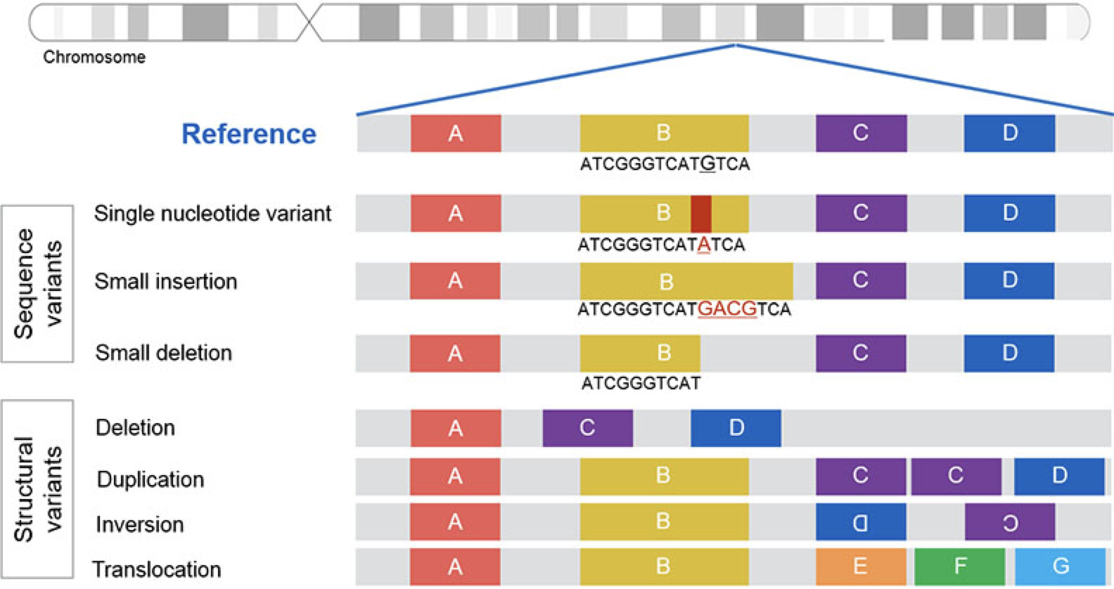 --- ## Why are we interested in differences? 1. Association with traits and phenotypes 2. $\ldots$ Notes: understanding gene function, understanding what makes us human, understanding human migration and human ancestry. --- ## SNVs * $N$ total reads * $N-K$ match the reference allele (A) * $K$ match the alternate allele (B) * Goal: classify each column as * homozygous reference (AA) * heterozygous (AB) * homozygous alternate (BB) Notes: What is the difference between SNV and SNP? --- ## SNVs * Method based on frequency threshold * $K/N$ in $[0, 0.2) \rightarrow$ homozygous reference * $K/N$ in $[0.2, 0.8) \rightarrow$ heterozygous * $K/N$ in $[0.8, 1.0] \rightarrow$ homozygous alternate * Thoughts? Note: Such heuristics were used in some of the earliest variant callers such as VarScan. Limitations include that this does not account for any sources of bias, assumes the separability of the three states, does not account for differences in copy number and assumes that the coverage is uniform, which rules out exome sequencing or amplicon sequencing and data from cancer genomes. --- 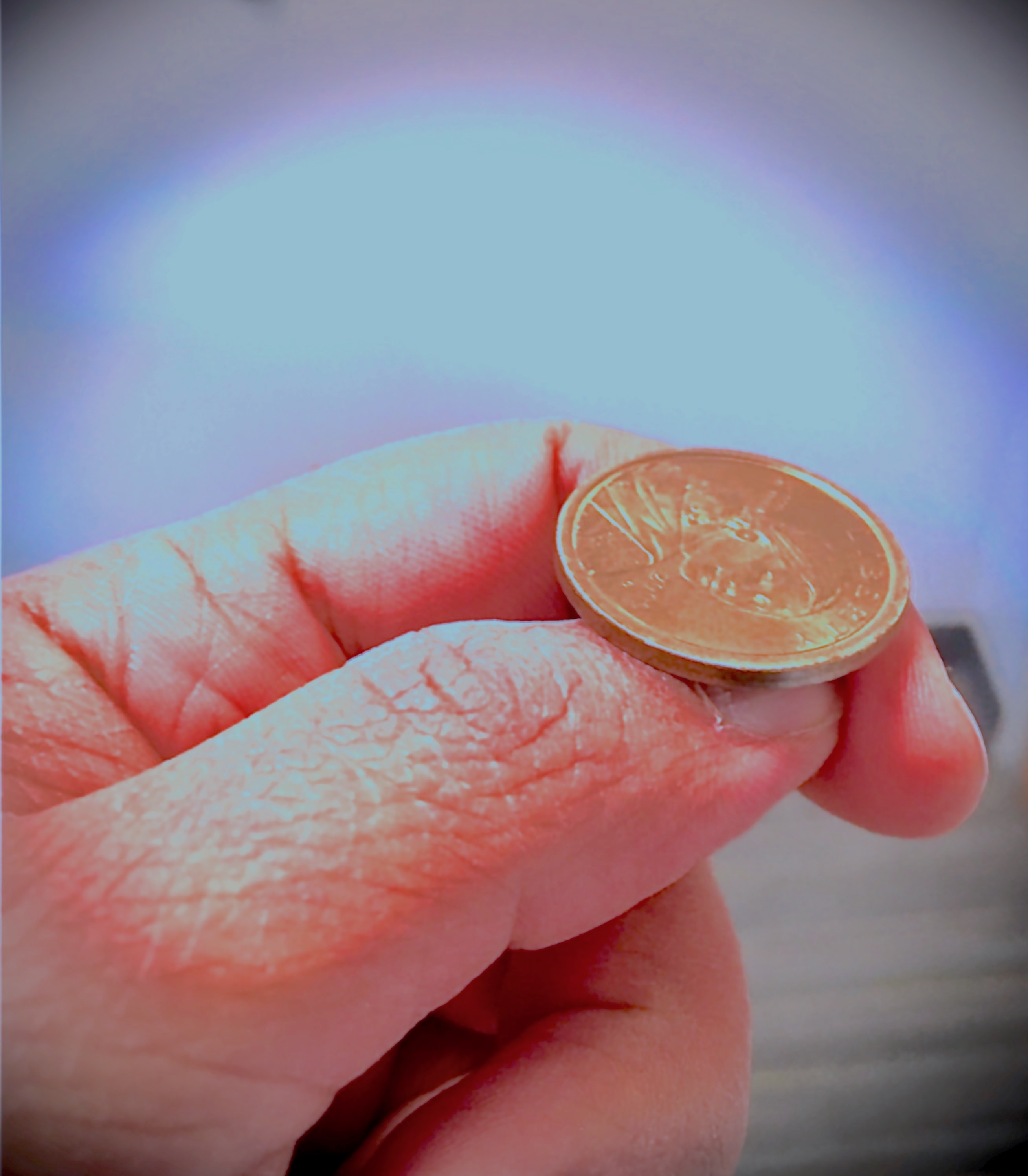 <!-- .element height="50%" width="50%" --> --- ## Revisiting binomial distribution * Coin flips: $P(H) = \mu$, $P(T) = 1-\mu$ * $X$ be the random variable representing the number of heads * $X$ has a binomial distribution, $X ∼ Bin(N, \mu)$ * Probability of exactly $k$ heads in $n$ trials $$P(X=k | N,\mu) = {n \choose k} \mu^k (1-\mu)^{n-k}$$ Note: The binomial distribution with parameters n and mu is the discrete probability distribution of the number of successes in a sequence of n independent yes (e.g., "heads" or "reference allele") or no (e.g., "tails", or "alternate allele") experiments, each of which yields success with probability mu. Remember we studied this in the statistical review. Now let's say that we have an observation of 59 H, 41 T, can we say something about mu? --- ## Estimating probabilities * Coin flips: $P(H) = \mu$, $P(T) = 1-\mu$ * We want to learn $\mu$ * Training data from $n$ flips * $\alpha_H + \alpha_T = n$ * What is $\hat{\mu}$? $$\hat{\mu} = \frac{\alpha_H}{\alpha_H + \alpha_T}$$ <!-- .element : class="fragment" data-fragment-index="1" --> Note: This approach is quite reasonable, and very intuitive. It is a good approach when we have plenty of training data. However, this can produce unreliable estimates when we have small amounts of data --- ## Maximum Likelihood Estimation ```R x <- seq(1,4000) data <- sample(c(0,1),length(x),replace=TRUE,prob=c(0.3,0.7)) mu <- rep(NA, length(x)) for (i in x) { mu[i] = sum(data[1:i])/i } plot(x, mu) abline(h=0.7) ``` 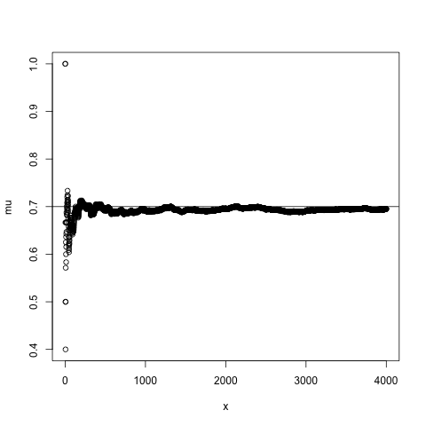 <!-- .element height="40%" width="40%" --> --- ## Maximum Likelihood Estimation ```R x <- seq(1,4000) data <- sample(c(0,1),length(x),replace=TRUE,prob=c(0.3,0.7)) mu <- rep(NA, length(x)) for (i in x) { mu[i] = sum(data[1:i])/i } plot(x, mu) abline(h=0.7) ``` 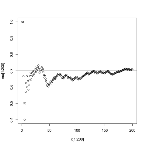 <!-- .element height="40%" width="40%" --> --- ## Including priors $$\hat{\mu} = \frac{\alpha_H + \gamma_H}{(\alpha_H + \gamma_H) + (\alpha_T + \gamma_T)}$$ * Incorporates our prior assumption in the ratio $\frac{\gamma_H}{\gamma_T}$ * We can express our degree of certainty of the priors by increasing $\gamma_H + \gamma_T$ * If $\gamma_H = \gamma_T = 0$, then this is the same as MLE --- ## Including priors ```R x <- seq(1,4000) data <- sample(c(0,1),length(x),replace=TRUE,prob=c(0.3,0.7)) gamma0 <- 50 gamma1 <- 50 mu <- rep(NA, length(x)) for (i in x) { mu[i] = (sum(data[1:i]) + gamma1)/(i + gamma0 + gamma1) } plot(x, mu, ylim=c(0,1)) abline(h=0.7) ``` 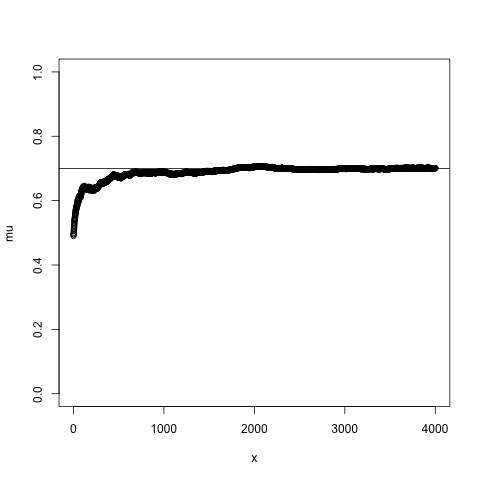 <!-- .element height="40%" width="40%" --> --- ## Including priors ```R x <- seq(1,4000) data <- sample(c(0,1),length(x),replace=TRUE,prob=c(0.3,0.7)) gamma0 <- 25 gamma1 <- 75 mu <- rep(NA, length(x)) for (i in x) { mu[i] = (sum(data[1:i]) + gamma1)/(i + gamma0 + gamma1) } plot(x, mu, ylim=c(0,1)) abline(h=0.7) ``` 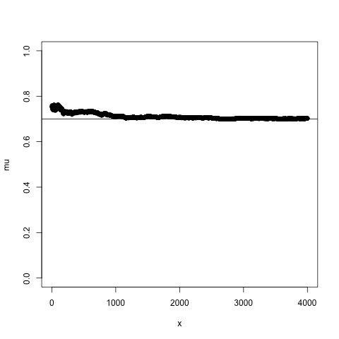 <!-- .element height="40%" width="40%" --> --- ## Maximum Likelihood Estimation $$\hat{\mu} = \arg \max_{\mu} P(D|\mu)$$ Note: The intuition underlying this principle is that we are more likely to observe data D if we are in a world where the appearance of this data is highly probable. Therefore, we should estimate \mu by assigning it whatever value maximizes the probability of having observed D. --- ## Maximum Likelihood Estimation $$P(D = \alpha_H, \alpha_T|\mu) = \mu^{\alpha_H} (1 - \mu)^{\alpha_T}$$ $$\begin{eqnarray} \hat{\mu} &=& \arg \max_{\mu} P(D|\mu) \\\\\\ &=& \arg \max_{\mu} ln\ P(D|\mu)\\\\\\ &=& \arg \max_{\mu} \ell(\mu) \end{eqnarray}$$ <!-- .element : class="fragment" data-fragment-index="1" --> Note: The quantity P(D|θ) is often called the data likelihood, or the data likelihood function because it expresses the probability of the observed data D as a function of θ. This likeli- hood function is often written L(θ) = P(D|θ). --- ## Maximum Likelihood Estimation $$\begin{eqnarray} \frac{\partial\ \ell(\mu)}{\partial \mu} &=& \frac{\partial\ ln\ P(D|\mu)}{\partial \mu}\\\\\\ &=& \frac{\partial\ ln\[\mu^{\alpha_H} (1 - \mu)^{\alpha_T}\]}{\partial \mu}\\\\\\ &=& \alpha_H \frac{\partial\ ln\ \mu}{\partial \mu} + \alpha_T \frac{\partial\ ln\ (1-\mu)}{\partial \mu}\\\\\\ &=& \alpha_H \frac{\partial\ ln\ \mu}{\partial \mu} + \alpha_T \frac{\partial\ ln\ (1-\mu)}{\partial (1- \mu)} \frac{\partial (1-\mu)}{\partial \mu}\\\\\\ &=& \alpha_H \frac{1}{\mu} - \alpha_T \frac{1}{1-\mu} \end{eqnarray}$$ Note: Set this to 0 and you will get your value for \hat{\mu} --- ## Maximum Likelihood Estimation $$\frac{\partial\ \ell(\mu)}{\partial \mu} = 0$$ $$\hat{\mu} = \frac{\alpha_H}{\alpha_H + \alpha_T}$$ <!-- .element : class="fragment" data-fragment-index="1" --> --- ## Maximum a Posteriori Estimation (MAP) $$\hat{\mu} = \arg \max_{\mu} P(\mu|D)$$ Note: we should choose the value of \mu that is most probable, given the observed data D and our prior assumptions summarized by P(\mu). --- ## Maximum a Posteriori Estimation (MAP) $$\begin{eqnarray} \hat{\mu} &=& \arg \max_{\mu} P(\mu|D)\\\\\\ &=& \arg \max_{\mu} \frac{P(D|\mu)P(\mu)}{P(D)}\\\\\\ &=& \arg \max_{\mu} P(D|\mu)P(\mu) \end{eqnarray}$$ Note: MLE looks to maximise P(D|\mu), but here we maximise that and our priors. P(D) is not dependent on \mu. --- ## Maximum a Posteriori Estimation (MAP) $P(\mu) = Beta(\beta_T, \beta_H) = \frac{\mu^{\beta_H-1} (1-\mu)^{\beta_T-1}}{B(\beta_T, \beta_H)}$ $$\begin{eqnarray} \hat{\mu} &=& \arg \max_{\mu} P(D|\mu)P(\mu)\\\\\\ &=& \arg \max_{\mu} \mu^{\alpha_H} (1 - \mu)^{\alpha_T} \frac{\mu^{\beta_H-1} (1-\mu)^{\beta_T-1}}{B(\beta_T, \beta_H)}\\\\\\ &=& \arg \max_{\mu} \mu^{\alpha_H+\beta_H-1} (1-\mu)^{\alpha_T+\beta_T-1} \end{eqnarray}$$ <!-- .element : class="fragment" data-fragment-index="1" --> Note: When data is generated by multiple i.i.d. draws of a Bernoulli random variable, the most common form of prior is a Beta distribution. Beta distribution has a functional form that is the same as the data likelihood P(D|θ) in our problem, so that when we multiply these two forms together to get the quantity P(D|θ)P(θ) , this product is easily expressed as yet another expression of this same functional form. The denominator is a normalization term which assures the probability integrates to one, but which is independent of \mu. --- ## Maximum a Posteriori Estimation (MAP) $$\hat{\mu} = \frac{\alpha_H + \beta_H - 1}{(\alpha_H + \beta_H - 1) + (\alpha_T+\beta_T-1)}$$ --- 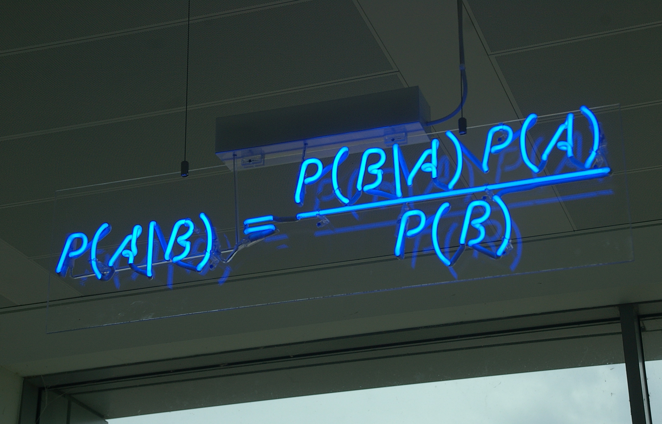 Note: Bayes' theorem spelt out in blue neon at the offices of HP Autonomy in Cambridge --- ## Bayes theorem * Consider a diagnostic test for prostate cancer * 1% of patients have PCa * 80% of the patients are diagnosed with PCa when they have it * 10% of the patients are diagnosed with PCa when they don't have it | | has PCa (1%) | doesn't have PCa | | ------------- | ------------ | ---------------- | | Test Positive | 80% | 10% | | Test Negative | 20% | 90% | --- ## Bayes theorem | | has PCa (1%) | doesn't have PCa (99%) | | ------------- | ------------ | ---------------- | | Test Positive | 80% | 10% | | Test Negative | 20% | 90% | What’s the chance a patient has PCa if they get a positive result? * Chance of a true positive = 0.008 * Chance of getting any type of positive result = 0.107 * Chance of the patient having CaP if they get a positive result = 0.008/0.107 = 7.47\% Note: Chance of a true positive = chance you have cancer * chance test caught it = 0.01 * 0.8 = 0.008. Chance of a false positive = 0.99 * 0.1 = 0.099. Chance of getting any type of positive result = chance of a true positive plus the chance of a false positive = 0.008 + 0.099 = 0.107 --- ## Bayes theorem $A,B$ = events, $P(B) \neq 0$<br> $P(A)$ = probability of observing $A$<br> $P(B)$ = probability of observing $B$<br> $P(B|A)$ = probability of event $B$ occurring given that $A$ is true<br> $P(A|B)$ = probability of event $A$ occurring given that $B$ is true<br> $$P(A|B) = \frac{P(B|A) . P(A)}{P(B)}$$ --- ## Bayes theorem: Bayesian interpretation * Probability : degree of belief * $P(A)$ = initial degree of belief in $A$ * $P(A|B)$ = degree of belief after incorporating that $B$ is true * $\frac{P(B|A)}{P(B)}$ = support B provides for $A$ $$P(A|B) = \frac{P(B|A) . P(A)}{P(B)}$$ Note: In the Bayesian interpretation, probability measures a "degree of belief". Bayes' theorem links the degree of belief in a proposition before and after accounting for evidence. ---  <!-- .element height="50%" width="50%" --> --- ## Binomial likelihood model * Suppose we run $T$ experiments where we toss the same coin $N={N_1,N_2,\ldots,N_T}$ times and come up with counts of heads $x = {x_1,x_2,\ldots,x_T}$ * Assume tosses are independent and identically distributed * What is the probability of observing the head counts given the coin and $\mu$? $$P(x_{1:T}|N_{1:T},\mu) = \prod_{i=1}^{T} Bin(x_i|N_i,\mu)$$ Note: We can read this as P(Data|\mu) --- ## Maximum likelihood estimation * What is $\mu$, given the evidence? * Likelihood $$P(x_{1:T}|N_{1:T},\mu) = \prod_{i=1}^{T} Bin(x_i|N_i,\mu)$$ --- ## Maximum likelihood estimation * What is $\mu$, given the evidence? * Log-likelihood $$log\ P(x_{1:T}|N_{1:T},\mu) = \sum_{i=1}^{T} log\ Bin(x_i|N_i,\mu)$$ --- ## Maximum likelihood estimation * What is $\mu$, given the evidence? * Log-likelihood $$log\ P(x_{1:T}|N_{1:T},\mu) = \sum_{i=1}^{T} log\ Bin(x_i|N_i,\mu)$$ * $\hat{\mu} = \frac{\sum_{i=1}^{T} x_i}{\sum_{i=1}^{T} N_i}$ Note: We can estimate this model parameter using MLE. Take log of the likelihood. Take the derivative wrt $\mu$. Equate it to 0. Solve for $\mu$ --- ## Maximum likelihood estimation ```code N = sample(1:200, 6, replace=TRUE) N ``` ```text [1] 191 99 22 63 144 84 ``` ```code x = c() for (i in N) { x = c(x, sum(rbinom(i, 1, prob=0.7))) } x ``` ```text [1] 133 71 14 47 97 67 ``` ```code mu = sum(x) / sum(N) mu ``` ```text [1] 0.7114428 ``` --- ## Priors * MLE uses the evidence to estimate parameters ($\mu$) * What if the sample size is small? Or we have missing data? * Prior distribution for binomial parameter $p$ * $\mu \in [0,1]$ and can be sampled from a distribution itself * $\mu \sim Beta(\alpha, \beta)$ * $P(\mu) = Beta(\mu | \alpha, \beta)$ Note: We might overfit the MLE. Why is that a problem? Can we capture a more natural expectation of how a coin might behave? Also, what if we have some knowledge that the coin might be biased? The beta distribution is a suitable model for the random behavior of percentages and proportions. \mu has a Beta distribution with parameters alpha and beta. The distribution is roughly centered on a/(a+b), The larger the values of a and b, the smaller the variance of the distribution about the mean. --- ## Bayesian statistics counts of heads $x = {1,2,\ldots,x_T}$ for $N={1,2,\ldots,N_T}$ times and a prior distribution on $\mu$ $$P(x_{1:T}|N_{1:T},\mu) = \prod_{i=1}^{T} Bin(x_i|N_i,\mu)$$ $P(\mu) = Beta(\mu | \alpha, \beta)$ We want $P(\mu | x)$, but we have $P(x|\mu)$ and $P(\mu)$ Note: So now we have the likelihood and the prior. We want the posterior, is our belief state by combining evidence from observations and our prior beliefs. --- ## Bayesian statistics counts of heads $x = {1,2,\ldots,x_T}$ for $N={1,2,\ldots,N_T}$ times and a prior distribution on $\mu$ $$P(x_{1:T}|N_{1:T},\mu) = \prod_{i=1}^{T} Bin(x_i|N_i,\mu)$$ $P(\mu) = Beta(\mu | \alpha, \beta)$ We want $P(\mu | x)$, but we have $P(x|\mu)$ and $P(\mu)$ $$P(\mu | x) \propto \prod_{i=1}^{T} Bin(x_i|N_i,\mu) \times Beta(\mu | \alpha, \beta)$$ --- ## Posterior for Beta-Binomial $$P(\mu | x) \propto \prod_{i=1}^{T} Bin(x_i|N_i,\mu) \times Beta(\mu | \alpha, \beta)$$ Beta is a [conjugate prior](https://stephens999.github.io/fiveMinuteStats/bayes_conjugate.html) for the binomial, the product of binomial and Beta has the form of a Beta $$\begin{eqnarray} P(\mu | x) &\propto& \prod_{i=1}^{T} Bin(x_i|N_i,\mu) \times Beta(\mu | \alpha, \beta) \\\\\\ &=& \prod_{i=1}^{T} Beta(\mu | x_i + \alpha, N_i - x_i + \beta ) \end{eqnarray}$$ Note: For some likelihood functions, if you choose a certain prior, the posterior ends up being in the same distribution as the prior. Such a prior then is called a Conjugate Prior. The Beta distribution is a conjugate prior for the Bernoulli, binomial, negative binomial and geometric distributions (seems like those are the distributions that involve success \& failure) --- ## MAP estimate $$\begin{eqnarray} P(\mu | x) &\propto& \prod_{i=1}^{T} Bin(x_i|N_i,\mu) \times Beta(\mu | \alpha, \beta) \\\\\\ &=& \prod_{i=1}^{T} Beta(\mu | x_i + \alpha, N_i - x_i + \beta ) \end{eqnarray}$$ What is $\mu$ for this coin given the evidence and the prior? * Maximum a posteriori estimate * Mode of $Beta(\alpha,\beta)$ is $\frac{\alpha − 1}{\alpha+\beta-2}$ * We have $\alpha' = \sum_i^T x_i + \alpha$ * We have $\beta' = \sum_i^T (N_i - x_i) + \beta$ Note: MAP refers to the mode of the posterior distribution and the mode of a Beta is --- ## Mapping mutation calling on sequencing data Suppose we run $T$ experiments where we toss the same coin $N={1,2,\ldots,N_T}$ times and come up with counts of heads $x = {1,2,\ldots,x_T}$. --- ## Using multiple coins Suppose we now have three types of coins $fair, heads, tails$. We still run $T$ experiments, but now each experiment involves first picking one of the three coins from a hat. * $N={N_1,N_2,\ldots,N_T}$ * $x = {x_1,x_2,\ldots,x_T}$ * We don't know the proportion of each coin type in the hat * We don’t know which coin was drawn for each experiment * We don't know $\mu$ for each type of coin --- ## Latent state model * What is the proportion of each coin type in the hat? * $\pi_k$ is the probability of drawing coin type $k$ * $\sum_{k=1}^{K} \pi_k= 1$ * Which coin did each referee draw? * Let $Z_i = k$ be the type of coin in the $i^{th}$ experiment * $Z_i$ is a latent variable such that $P(Z_i = k | \pi_{1:K}) = \pi_k$ * Proportions $\pi_k$ of the coin types follows a Dirichlet distribution, so $P(\pi_{1:K}|\delta_{1:K}) = Dirichlet(\pi_{1:K}|\delta_{1:K})$ Note: K is the number of coin types. Dirichlet distribution is a conjugate prior of the categorical distribution. \delta_i is the concentration parameters and all > 0. --- ## Mixture of binomials * What is the $\mu$ for each type of coin * For a single coin, $P(x_i | N_i, \mu) = Bin(x_i | N_i, \mu)$ * Define the likelihood for a 3-component mixture of binomials with 3 parameters $\mu_{1:K}$ ($\mu_{fair}, \mu_{heads}, \mu_{tails}$) * Observed likelihood $$P(x_i | Z_i=k, N_i, \mu_{1:K}) = Bin(x_i | N_i, \mu_k)$$ * Mixture model $$P(x_i | N_i, \mu_{1:K}, \pi_{1:K}) = \sum_{k=1}^{K} \pi_k Bin(x_i | N_i, \mu_k)$$ $$P(\mu_k | \alpha_k, \beta_k) = Beta(\mu_k | \alpha_k, \beta_k)$$ --- ## Likelihood as a mixture of binomials Likelihood Function of the Model $$L(x_{1:T},N_{1:T} | \mu_{1:K}, \pi_{1:K}) = \prod_{i=1}^{T} \sum_{k=1}^{K} \pi_k Bin(x_i | N_i, \mu_k)$$ Log-likelihood $$\ell = \sum_{i=1}^{T} \Big( \sum_{k=1}^{K} \pi_k Bin(x_i | N_i, \mu_k)\Big) $$ Note: MLE is normally done by taking the derivative of the data likelihood P(X) with respect to the model parameter θ and solving the equation. However, in some cases where we have hidden (unobserved) variables in the model, the derivative w.r.t. the model parameter does not have a closed form solution, which is another way of saying that we cannot express the solution in terms of well known and accepted functions. --- ## Mixture Model: using EM * Initialize parameters: $\pi_{1:K}$ and $\mu_{1:K}$ * E-Step: compute "responsibilities" * Which coin is responsible for generating observation $x_i$ * M-Step: Update parameters * What is the proportion of each coin type in the hat? $\pi_{1:K}$ * What is the prob. of heads for each coin type? $\mu_{1:K}$ * Iterate between E-Step and M-Step, check when log-likelihood $\ell$ stops increasing. --- ## E-Step Which coin is responsible for generating observation $x_i$ $$\begin{eqnarray} P(Z_i=k|x_i,N_i,\pi_{1:K},\mu_{1:K}) &=& \frac{p(x_i|Z_i=k)p(Z_i=k)}{p(x_i)} \\\\\\ &=& \frac{\pi_k Bin(x_i|N_i,\mu_k)}{\sum_{k'=1}^{K} \pi_k'Bin(x_i|N_i,\mu_k')} \\\\\\ &=& \gamma(Z_i=k) \end{eqnarray}$$ Note: this gives you a Posterior distribution of the latent variables which can be thought of as a matrix with T rows and K columns. So you now have a probability of each coin type to have been used for each of the T experiments --- ## M-Step What is the proportion of each coin type? $$\hat{\pi_k} = \frac{\sum_{i=1}^{T} \gamma(Z_i=k) + \delta(k) - 1}{\sum_{j=1}^{K} \sum_{i=1}^{T} \gamma(Z_i=j) + \delta(j) - 1} $$ What is the prob. of heads for each coin type? $$\hat{\mu_k} = \frac{\sum_{i=1}^{T} \gamma(Z_i=k)x_i + \alpha_k - 1}{\sum_{i=1}^{T} \gamma(Z_i=j)N_i + \alpha_k + \beta_k- 2} $$ Note: both are MAP values. --- ## EM algorithm Log-posterior = Log-likelihood + Log priors Log-likelihood = $\sum_{i=1}^T log\ \big( \sum_{k=1}^K \hat{\pi_k} Bin(x_i|N_i,\hat{\mu_k})\big)$ Log priors = $Dir(\hat{\pi}|\delta) + \sum_{k=1}^K log\ Beta(\hat{\mu_k}|\alpha_k, \beta_k)$ * More on Mixture models and EM * Christopher M. Bishop. Pattern Recognition and Machine Learning (Chapter 9) * Kevin P. Murphy. Machine Learning (Chapter 3) --- ## More on mixture modeling * [Mixture models](https://stephens999.github.io/fiveMinuteStats/mixture_models_01.html) * [EM algorithm](https://stephens999.github.io/fiveMinuteStats/em_algorithm_01.html) * [Variational view of the EM algorithm](https://stephens999.github.io/fiveMinuteStats/em_variational.html) * [Gaussian mixture models](https://stephens999.github.io/fiveMinuteStats/intro_to_em.html) --- ## Mapping mutation calling on sequencing data Suppose we run $T$ experiments where we first select one of 3 coins and then toss the coin $N={N_1,N_2,\ldots,N_T}$ times and come up with counts of heads $x = {x_1,x_2,\ldots,x_T}$. --- ## Mapping mutation calling on sequencing data Suppose we run $T$ experiments where we first select one of 3 coins and then toss the coin $N={N_1,N_2,\ldots,N_T}$ times and come up with counts of heads $x = {x_1,x_2,\ldots,x_T}$. * Genomic loci $1,\ldots,T$. * For each locus $i$ * Depth (total reads): $N_i$, Count of reference base: $x_i$, Count of variant base: $N_i − x_i$ * Parameters * Probability of genotypes: $\pi_{AA}, \pi_{AB}, \pi_{BB}$, Probability of reference base for 3 genotypes: $\mu_{AA}, \mu_{AB}, \mu_{BB}$ * Latent variable * Probability that locus $i$ has genotype $k: \gamma(Z_i = k)$ --- ## SNVs $$P(G|D) = \frac{P(D|G).P(G)}{P(D)}$$ * $G$ = genotype ($AA,AB,BB$) * $D$ = data (bases from reads aligning to that locus) * $P(G|D)$ = posterior, probability of a given genotype, given the observed data * $P(D|G)$ = likelihood, probability of the data, given an underlying genotype * $P(D)$ = prior, probability to observe a given genotype --- ## SNV calling * Maximum likelihood : find assignment for $G$ that maximizes the likelihood $P(D|G)$ * GATK * Maximum a posteriori: find assignment for $G$ that maximizes the posterior $P(G|D)$ * MAQ, FreeBayes --- ## Other factors? What other factors can influence this distribution? * Depth of coverage at the locus * Quality of bases at the locus * Mapping quality at the locus * Sequencing bias * Expected polymorphism rate at the locus --- ## Extending the model (FreeBayes) $G$ = genotypes<br> $R$ = reads<br> $S$ = locus is well-characterized/mapped $$P(G,S|R) = \frac{P(R|G,S) P(G)P(S)} {P(R)}$$ * $P(R|G,S)$ is data likelihood * $P(G)$ is prior estimate of the genotypes * $P(S)$ is prior estimate of the mappability of the locus * $P(R)$ is a normalizer --- ## Extending the model (FreeBayes) $$P(G,S|R) = \frac{P(R|G,S) P(G)P(S)} {P(R)}$$ 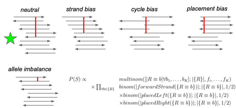 --- ## What about indels * Small indels (< 50 bps) * Intermediate sized indels (50 - 250 bps) * Large indels (> 250 bps) 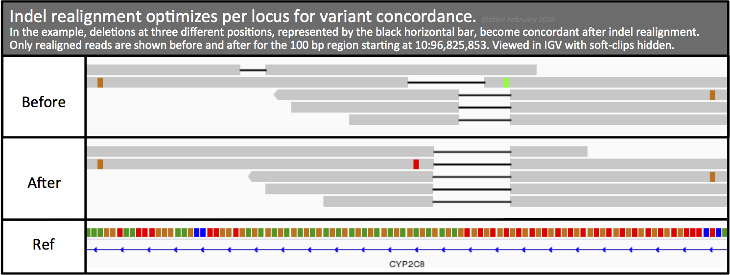 <!-- .element: class="fragment" data-fragment-index="1" --> [GATK Docs](https://github.com/broadinstitute/gatk-docs/blob/master/gatk3-tutorials/(howto)_Perform_local_realignment_around_indels.md) --- ## Small indels 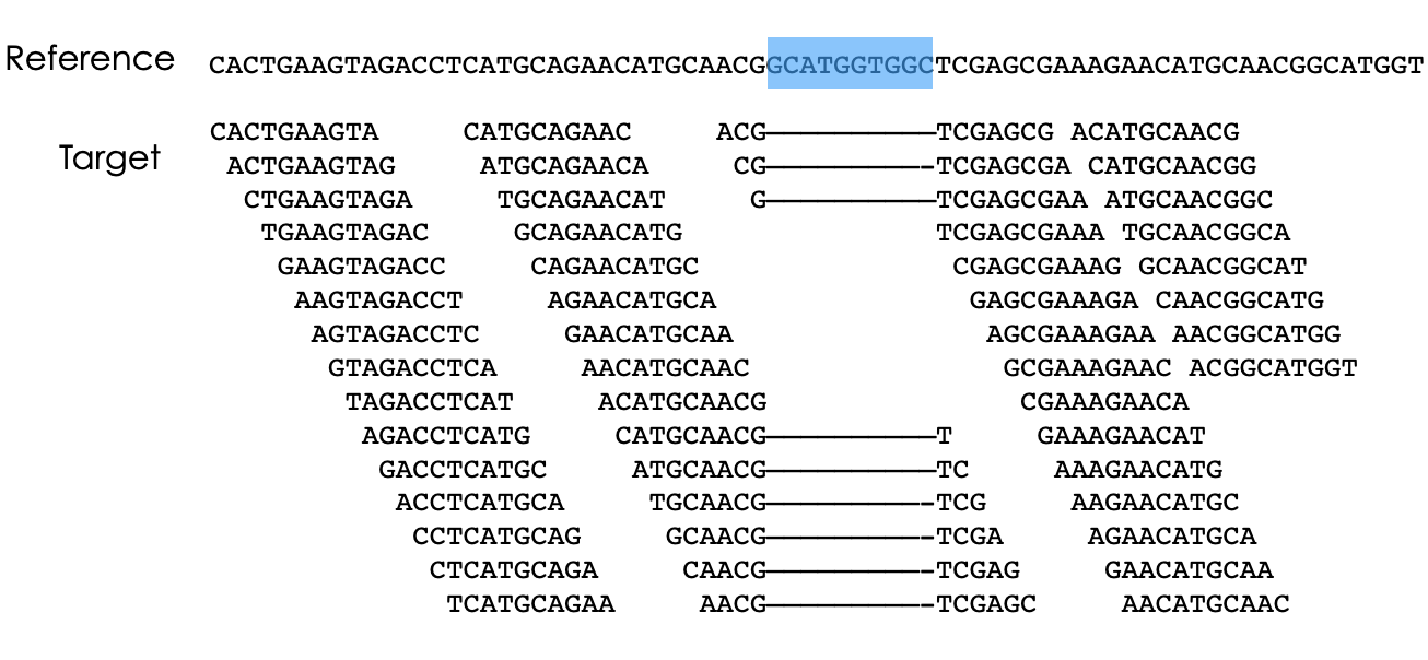 Note: for medium sized indels we have to move to assembly and haplotype- driven detection and we will cover some of that in the genome assembly lecture, but the big idea is that we use the alignments to localize reads, then process them again with assembly approaches to determine candidate alleles. Another point is that we see several sources of evidence that are at play in this. Explain SR and RD. --- ## Paired-end reads  <small>[Advantages of paired-end and single-read sequencing](https://emea.illumina.com/science/technology/next-generation-sequencing/plan-experiments/paired-end-vs-single-read.html)</small> --- ## Paired-end reads 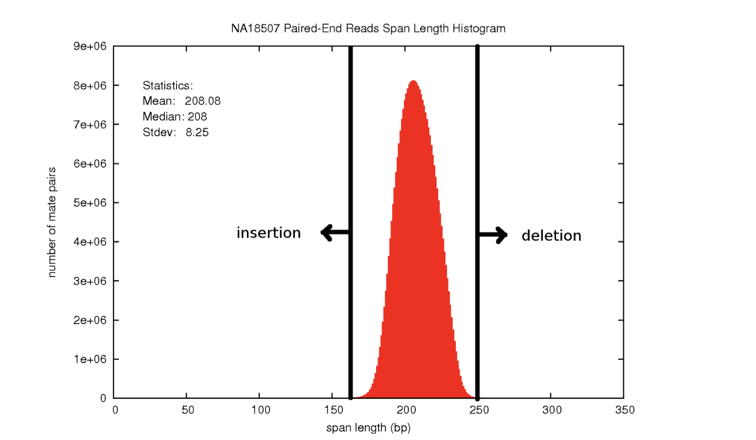 <small>[PMC2704429](https://pubmed.ncbi.nlm.nih.gov/19447966/)</small> --- ## Large deletions  --- ## Large deletions  --- ## Large deletions  --- ## Large deletions  --- ## Large deletions  --- ## Large deletions  --- ## Large deletions  --- ## Large deletions  --- ## Large deletions  --- ## Structural variants  <!-- .element height="70%" width="70%" --> <small>[PMC6868818](https://www.ncbi.nlm.nih.gov/pmc/articles/PMC6868818/)</small> ---