Data Wrangling and Analyses with Tidyverse

Estimated time: 55 minutes

Overview

Questions

• How can I manipulate data frames without repeating myself?

Objectives

• Describe what the dplyr package in R is used for.
• Apply common dplyr functions to manipulate data in R.
• Employ the ‘pipe’ operator to link together a sequence of functions.
• Employ the ‘mutate’ function to apply other chosen functions to existing columns and create new columns of data.
• Employ the ‘split-apply-combine’ concept to split the data into groups, apply analysis to each group, and combine the results.

Bracket subsetting is handy, but it can be cumbersome and difficult to read, especially for complicated operations.

Luckily, the dplyr package provides a number of very useful functions for manipulating data frames in a way that will reduce repetition, reduce the probability of making errors, and probably even save you some typing. As an added bonus, you might even find the dplyr grammar easier to read.

Here we’re going to cover some of the most commonly used functions as well as using pipes (%>%) to combine them:

1. glimpse()
2. select()
3. filter()
4. group_by()
5. summarize()
6. mutate()
7. pivot_longer and pivot_wider

Packages in R are sets of additional functions that let you do more stuff in R. The functions we’ve been using, like str(), come built into R; packages give you access to more functions. You need to install a package and then load it to be able to use it. For this lesson, we have installed all the packages for you, so you should be able to load them for use

R

library("dplyr")          ## loads in dplyr package to use
library("tidyr")          ## loads in tidyr package to use
library("ggplot2")          ## loads in ggplot2 package to use
library("readr")          ## load in readr package to use

You only need to install a package once per computer, but you need to load it every time you open a new R session and want to use that package.

What is dplyr?

---

The package dplyr is a fairly new (2014) package that tries to provide easy tools for the most common data manipulation tasks. This package is also included in the tidyverse package, which is a collection of eight different packages (dplyr, ggplot2, tibble, tidyr, readr, purrr, stringr, and forcats). It is built to work directly with data frames. The thinking behind it was largely inspired by the package plyr which has been in use for some time but suffered from being slow in some cases.dplyr addresses this by porting much of the computation to C++. An additional feature is the ability to work with data stored directly in an external database. The benefits of doing this are that the data can be managed natively in a relational database, queries can be conducted on that database, and only the results of the query returned.

This addresses a common problem with R in that all operations are conducted in memory and thus the amount of data you can work with is limited by available memory. The database connections essentially remove that limitation in that you can have a database that is over 100s of GB, conduct queries on it directly and pull back just what you need for analysis in R.

Loading .csv files in tidy style

The Tidyverse’s readr package provides its own unique way of loading .csv files in to R using read_csv(), which is similar to read.csv(). read_csv() allows users to load in their data faster, doesn’t create row names, and allows you to access non-standard variable names (ie. variables that start with numbers of contain spaces), and outputs your data on the R console in a tidier way. In short, it’s a much friendlier way of loading in potentially messy data.

Now let’s load our vcf .csv file using read_csv():

R

variants <- read_csv("combined_tidy_vcf.csv") 

Taking a quick look at data frames

Similar to str(), which comes built into R, glimpse() is a dplyr function that (as the name suggests) gives a glimpse of the data frame.

R

glimpse(variants)

In the above output, we can already gather some information about variants, such as the number of rows and columns, column names, type of vector in the columns, and the first few entries of each column. Although what we see is similar to outputs of str(), this method gives a cleaner visual output.

Selecting columns and filtering rows

To select columns of a data frame, use select(). The first argument to this function is the data frame (variants), and the subsequent arguments are the columns to keep.

R

select(variants, sample_id, REF, ALT, DP)

To select all columns except certain ones, put a “-” in front of the variable to exclude it.

R

select(variants, -CHROM)

dplyr also provides useful functions to select columns based on their names. For instance, ends_with() allows you to select columns that ends with specific letters. For instance, if you wanted to select columns that end with the letter “B”:

R

select(variants, ends_with("B"))

Challenge

Challenge

Create a table that contains all the columns with the letter “i” and column “POS”, without columns “Indiv” and “FILTER”. Hint: look at for a function called contains(), which can be found in the help documentation for ends with we just covered (?ends_with). Note that contains() is not case sensistive.

Show me the solution

R

# First, we select "POS" and all columns with letter "i". This will contain columns Indiv and FILTER. 
variants_subset <- select(variants, POS, contains("i"))
# Next, we remove columns Indiv and FILTER
variants_result <- select(variants_subset, -Indiv, -FILTER)
variants_result

Challenge

Challenge (continued)

We can also get to variants_result in one line of code:

Alternative solution

R

variants_result <- select(variants, POS, contains("i"), -Indiv, -FILTER)
variants_result

To choose rows, use filter():

R

filter(variants, sample_id == "SRR2584863")

filter() will keep all the rows that match the conditions that are provided. Here are a few examples:

R

# rows for which the reference genome has T or G
filter(variants, REF %in% c("T", "G"))
# rows that have TRUE in the column INDEL
filter(variants, INDEL)
# rows that don't have missing data in the IDV column
filter(variants, !is.na(IDV))

We have a column titled “QUAL”. This is a Phred-scaled confidence score that a polymorphism exists at this position given the sequencing data. Lower QUAL scores indicate low probability of a polymorphism existing at that site. filter() can be useful for selecting mutations that have a QUAL score above a certain threshold:

R

# rows with QUAL values greater than or equal to 100
filter(variants, QUAL >= 100)

filter() allows you to combine multiple conditions. You can separate them using a , as arguments to the function, they will be combined using the & (AND) logical operator. If you need to use the | (OR) logical operator, you can specify it explicitly:

R

# this is equivalent to:
#   filter(variants, sample_id == "SRR2584863" & QUAL >= 100)
filter(variants, sample_id == "SRR2584863", QUAL >= 100)
# using `|` logical operator
filter(variants, sample_id == "SRR2584863", (MQ >= 50 | QUAL >= 100))

Challenge

Challenge

Select all the mutations that occurred between the positions 1e6 (one million) and 2e6 (inclusive) that have a QUAL greater than 200, and exclude INDEL mutations. Hint: to flip logical values such as TRUE to a FALSE, we can use to negation symbol “!”. (eg. !TRUE == FALSE).

Show me the solution

R

filter(variants, POS >= 1e6 & POS <= 2e6, QUAL > 200, !INDEL)

ERROR

Error: object 'variants' not found

Pipes

But what if you wanted to select and filter? We can do this with pipes. Pipes, are a fairly recent addition to R. Pipes let you take the output of one function and send it directly to the next, which is useful when you need to many things to the same data set. It was possible to do this before pipes were added to R, but it was much messier and more difficult. Pipes in R look like %>% and are made available via the magrittr package, which is installed as part of dplyr.

R

variants %>%
  filter(sample_id == "SRR2584863") %>%
  select(REF, ALT, DP)

In the above code, we use the pipe to send the variants data set first through filter(), to keep rows where sample_id matches a particular sample, and then through select() to keep only the REF, ALT, and DP columns. Since %>% takes the object on its left and passes it as the first argument to the function on its right, we don’t need to explicitly include the data frame as an argument to the filter() and select() functions any more.

Some may find it helpful to read the pipe like the word “then”. For instance, in the above example, we took the data frame variants, then we filtered for rows where sample_id was SRR2584863, then we selected the REF, ALT, and DP columns. The dplyr functions by themselves are somewhat simple, but by combining them into linear workflows with the pipe, we can accomplish more complex manipulations of data frames.

If we want to create a new object with this smaller version of the data we can do so by assigning it a new name:

R

SRR2584863_variants <- variants %>%
  filter(sample_id == "SRR2584863") %>%
  select(REF, ALT, DP)

This new object includes all of the data from this sample. Let’s look at just the first six rows to confirm it’s what we want:

R

SRR2584863_variants

Similar to head() and tail() functions, we can also look at the first or last six rows using tidyverse function slice(). Slice is a more versatile function that allows users to specify a range to view:

R

SRR2584863_variants %>% slice(1:6)

R

SRR2584863_variants %>% slice(10:25)

Challenge

Exercise: Pipe and filter

Starting with the variants data frame, use pipes to subset the data to include only observations from SRR2584863 sample, where the filtered depth (DP) is at least 10. Showing only 5th through 11th rows of columns REF, ALT, and POS.

Show me the solution

R

 variants %>%
 filter(sample_id == "SRR2584863" & DP >= 10) %>%
 slice(5:11) %>%
 select(sample_id, DP, REF, ALT, POS)

Mutate

Frequently you’ll want to create new columns based on the values in existing columns, for example to do unit conversions or find the ratio of values in two columns. For this we’ll use the dplyr function mutate().

For example, we can convert the polymorphism confidence value QUAL to a probability value according to the formula:

Probability = 1- 10 ^ -(QUAL/10)

We can use mutate to add a column (POLPROB) to our variants data frame that shows the probability of a polymorphism at that site given the data.

R

variants %>%
  mutate(POLPROB = 1 - (10 ^ -(QUAL/10)))

Challenge

Exercise

There are a lot of columns in our data set, so let’s just look at the sample_id, POS, QUAL, and POLPROB columns for now. Add a line to the above code to only show those columns.

Show me the solution

R

variants %>%
 mutate(POLPROB = 1 - 10 ^ -(QUAL/10)) %>%
 select(sample_id, POS, QUAL, POLPROB)

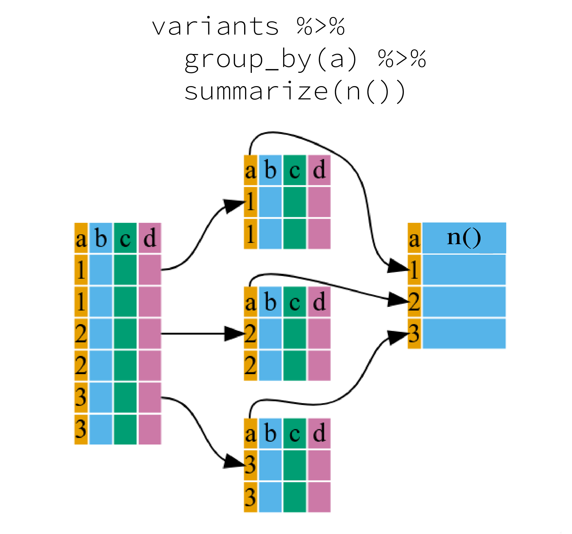
group_by() and summarize() functions

Many data analysis tasks can be approached using the “split-apply-combine” paradigm: split the data into groups, apply some analysis to each group, and then combine the results. dplyr makes this very easy through the use of the group_by() function, which splits the data into groups.

We can use group_by() to tally the number of mutations detected in each sample using the function tally():

R

variants %>%
  group_by(sample_id) %>%
  tally()

Since counting or tallying values is a common use case for group_by(), an alternative function was created to bypasses group_by() using the function count():

R

variants %>%
  count(sample_id)

Challenge

Challenge

• How many mutations are INDELs?

Show me the solution

R

variants %>%
  count(INDEL)

When the data is grouped, summarize() can be used to collapse each group into a single-row summary. summarize() does this by applying an aggregating or summary function to each group.

It can be a bit tricky at first, but we can imagine physically splitting the data frame by groups and applying a certain function to summarize the data.

¹

We can also apply many other functions to individual columns to get other summary statistics. For example,we can use built-in functions like mean(), median(), min(), and max(). These are called “built-in functions” because they come with R and don’t require that you install any additional packages. By default, all R functions operating on vectors that contains missing data will return NA. It’s a way to make sure that users know they have missing data, and make a conscious decision on how to deal with it. When dealing with simple statistics like the mean, the easiest way to ignore NA (the missing data) is to use na.rm = TRUE (rm stands for remove).

So to view the mean, median, maximum, and minimum filtered depth (DP) for each sample:

R

variants %>%
  group_by(sample_id) %>%
  summarize(
    mean_DP = mean(DP),
    median_DP = median(DP),
    min_DP = min(DP),
    max_DP = max(DP))

Callout

Grouped Data Frames in Tidyverse

When you group a data frame with group_by(), you get a grouped data frame. This is a special type of data frame that has all the properties of a regular data frame but also has an additional attribute that describes the grouping structure. The primary advantage of a grouped data frame is that it allows you to work with each group of observations as if they were a separate data frame.

Operations like summarise() and mutate() will be applied to each group separately. This is particularly useful when you want to perform calculations on subsets of your data.

To remove the grouping structure from a grouped data frame, you can use the ungroup() function. This will return a regular data frame.

For more details, refer to the dplyr documentation on grouping.

Reshaping data frames

It can sometimes be useful to transform the “long” tidy format, into the wide format. This transformation can be done with the pivot_wider() function provided by the tidyr package (also part of the tidyverse).

pivot_wider() takes a data frame as the first argument, and two arguments: the column name that will become the columns and the column name that will become the cells in the wide data.

R

variants_wide <- variants %>%
  group_by(sample_id, CHROM) %>%
  summarize(mean_DP = mean(DP)) %>%
  pivot_wider(names_from = sample_id, values_from = mean_DP)
variants_wide

The opposite operation of pivot_wider() is taken care by pivot_longer(). We specify the names of the new columns, and here add -CHROM as this column shouldn’t be affected by the reshaping:

R

variants_wide %>%
  pivot_longer(-CHROM, names_to = "sample_id", values_to = "mean_DP")

Resources

• Handy dplyr cheatsheet

• Much of this lesson was copied or adapted from Jeff Hollister’s materials

Key Points

• Use the dplyr package to manipulate data frames.
• Use glimpse() to quickly look at your data frame.
• Use select() to choose variables from a data frame.
• Use filter() to choose data based on values.
• Use mutate() to create new variables.
• Use group_by() and summarize() to work with subsets of data.

---

1. The figure was adapted from the Software Carpentry lesson, R for Reproducible Scientific Analysis↩︎